
Introduction
In this article, we will go through the tutorial for Keras Normalization Layer where will understand why a normalization layer is needed. We will also see what are the two types of normalization layers in Keras – i) Batch Normalization Layer and ii) Layer Normalization Layer and understand them in detail with the help of examples. We will finally do a comparison between batch normalization vs layer normalization with their advantages and disadvantages.
But before going into that let us first understand why Normalization is needed in the first place.
What is Normalization?
Normalization is a method usually used for preparing data before training the model. The main purpose of normalization is to provide a uniform scale for numerical values. If the dataset contains numerical data varying in a huge range, it will skew the learning process, resulting in a bad model. The normalization method ensures there is no loss of information and even the range of values isn’t affected.
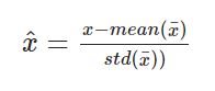
Normalization is done by the below formula, by subtracting the mean and dividing by the standard deviation.
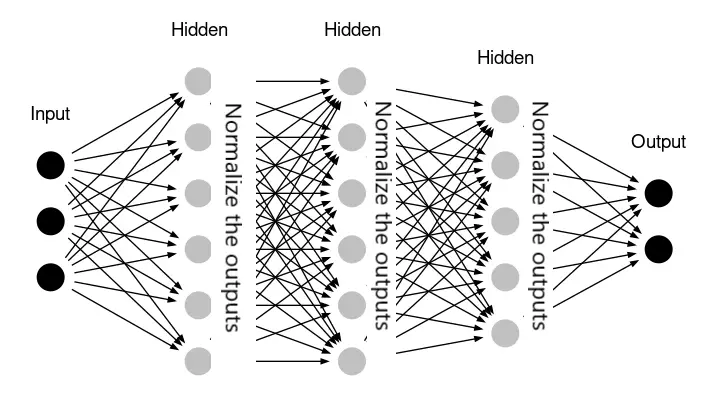
In spite of normalizing the input data, the value of activations of certain neurons in the hidden layers can start varying across a wide scale during the training process. This means the input to the neurons to the next hidden layer will also range across the wide range, bringing instability.
To deal with this problem, we use the techniques of “batch normalization” layer and “layer normalization” layer. Let us see these two techniques in detail along with their implementation examples in Keras.
Batch Normalization Layer
Batch Normalization Layer is applied for neural networks where the training is done in mini-batches. We divide the data into batches with a certain batch size and then pass it through the network. Batch normalization is applied on the neuron activation for all the samples in the mini-batch such that the mean of output lies close to 0 and the standard deviation lies close to 1. It also introduces two learning parameters gama and beta in its calculation which are all optimized during training.
Advantages of Batch Normalization Layer
- Batch normalization improves the training time and accuracy of the neural network.
- It decreases the effect of weight initialization.
- It also adds a regularization effect on the network.
- It works better with the fully Connected Neural Network (FCN) and Convolutional Neural Network.
Disadvantages of Batch Normalization Layer
- Batch normalization is dependent on mini-batch size which means if the mini-batch size is small, it will have little to no effect
- If there is no batch size involved, like in traditional gradient descent learning, we cannot use it at all.
- Batch normalization does not work well with Recurrent Neural Networks (RNN)
Syntax for Batch Normalization Layer in Keras
tf.keras.layers.BatchNormalization(
axis=-1,
momentum=0.99,
epsilon=0.001,
center=True,
scale=True,
beta_initializer="zeros",
gamma_initializer="ones",
moving_mean_initializer="zeros",
moving_variance_initializer="ones",
beta_regularizer=None,
gamma_regularizer=None,
beta_constraint=None,
gamma_constraint=None,
renorm=False,
renorm_clipping=None,
renorm_momentum=0.99,
fused=None,
trainable=True,
virtual_batch_size=None,
adjustment=None,
name=None,
**kwargs)
Keras Batch Normalization Layer Example
In this example, we’ll be looking at how batch normalization layer is implemented.
First, we load the libraries and packages that are required. We also import kmnist dataset for our implementation.
Install Keras Dataset
! pip install extra_keras_datasets
Import Libraries
from extra_keras_datasets import kmnist
import tensorflow
from tensorflow.keras.models import Sequential
from tensorflow.keras.layers import Dense, Flatten
from tensorflow.keras.layers import Conv2D, MaxPooling2D
from tensorflow.keras.layers import BatchNormalization
Model Configuration
In the below code snippet we are specifying the batch size as 250, the number of epochs executed is 25, the data will be classified into 10 different classes, 20% of the training data is used as the validation set and lastly, verbosity is set to true.
# Model configuration
batch_size = 250
no_epochs = 25
no_classes = 10
validation_split = 0.2
verbosity = 1
Download and Load Dataset
Next, we load the MNIST dataset from Keras datasets module.
# Load KMNIST dataset
(input_train, target_train), (input_test, target_test) = kmnist.load_data(type='kmnist')
Here we process the data, this helps it in preparing data for training.
# Shape of the input sets
input_train_shape = input_train.shape
input_test_shape = input_test.shape
Now we are obtaining the shape of both training and testing datasets. We also set the shape of keras input data.
# Keras layer input shape
input_shape = (input_train_shape[1], input_train_shape[2], 1)
To include channels during training, we are using the below code. There are instances when there are no apt channels, so we need to reshape the data for including those channels.
# Reshape the training data to include channels
input_train = input_train.reshape(input_train_shape[0], input_train_shape[1], input_train_shape[2], 1)
input_test = input_test.reshape(input_test_shape[0], input_test_shape[1], input_test_shape[2], 1)
The pre-processing of data is almost completed, we just need to convert data type to float32 format, it definitely makes the process faster.
# Parse numbers as floats
input_train = input_train.astype('float32')
input_test = input_test.astype('float32')
At last, we normalize the data for better results.
# Normalize input data
input_train = input_train / 255
input_test = input_test / 255
Designing the model architecture
In this section, we will be designing our neural network using the Sequential API of Keras. Notice we have used batch normalization layers in the design. Along with that, we have also used dense, convolutional, and pooling layers in the architecture.
# Create the model
model = Sequential()
model.add(Conv2D(32, kernel_size=(3, 3), activation='relu', input_shape=input_shape))
model.add(BatchNormalization())
model.add(MaxPooling2D(pool_size=(2, 2)))
model.add(BatchNormalization())
model.add(Conv2D(64, kernel_size=(3, 3), activation='relu'))
model.add(BatchNormalization())
model.add(MaxPooling2D(pool_size=(2, 2)))
model.add(BatchNormalization())
model.add(Flatten())
model.add(Dense(256, activation='relu'))
model.add(BatchNormalization())
model.add(Dense(no_classes, activation='softmax'))
Model compilation & fitting data
Now we need to compile our model. Model Compilation helps in instantiating the model architecture. In this step we are using sparse categorical crossentropy loss, adam optimizer is used for model optimization.
# Compile the model
model.compile(loss=tensorflow.keras.losses.sparse_categorical_crossentropy,
              optimizer=tensorflow.keras.optimizers.Adam(),
              metrics=['accuracy'])
Training the Model
At last, we are fitting the data to our model for training.
Here the input training set is provided corresponding targets, and then it is trained to pre-decided batch_size and number of epochs.
# Fit data to model
history = model.fit(input_train, target_train,
            batch_size=batch_size,
            epochs=no_epochs,
            verbose=verbosity,
            validation_split=validation_split)
Generating evaluation metrics
Now we will evaluate the performance of our model.
# Generate generalization metric  s
score = model.evaluate(input_test, target_test, verbose=0)
print(f'Test loss: {score[0]} / Test accuracy: {score[1]}')
Layer Normalization Layer
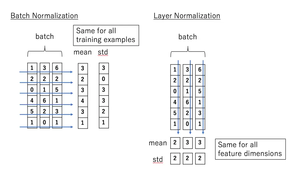
The next type of normalization layer in Keras is Layer Normalization which addresses the drawbacks of batch normalization. This technique is not dependent on batches and the normalization is applied on the neuron for a single instance across all features. Here also mean activation remains close to 0 and mean standard deviation remains close to 1.
Advantages of Layer Normalization
- It is not dependent on any batch sizes during training.
- It works better with Recurrent Neural Network.
Disadvantages of Layer Normalization
- It may not produce good results with Convolutional Neural Networks (CNN)
Syntax of Layer Normalization Layer in Keras
tf.keras.layers.LayerNormalization(
 axis=-1,
 epsilon=0.001,
 center=True,
 scale=True,
 beta_initializer="zeros",
 gamma_initializer="ones",
 beta_regularizer=None,
 gamma_regularizer=None,
 beta_constraint=None,
 gamma_constraint=None,
 trainable=True,
 name=None,
**kwargs)
Keras Normalization Layer Example
Let us see the example of how does LayerNormalization works in Keras. For this, we will be using the same dataset that we had used in the above example of batch normalization. Hence we are skipping the data download and preprocessing part for which you can refer to the above example. We will directly go to designing and training the neural network.
Designing the model architecture
import tensorflow as tf
model_lay = tf.keras.models.Sequential([
  # Reshape into "channels last" setup.
  tf.keras.layers.Reshape((28,28,1), input_shape=(28,28)),
  tf.keras.layers.Conv2D(filters=10, kernel_size=(3,3),data_format="channels_last"),
  # LayerNorm Layer
  tf.keras.layers.LayerNormalization(axis=3 , center=True , scale=True),
  tf.keras.layers.Flatten(),
  tf.keras.layers.Dense(128, activation='relu'),
  tf.keras.layers.Dropout(0.2),
  tf.keras.layers.Dense(10, activation='softmax')
])
Compiling the Model
# Compiling Layer Normalization Model
model_lay.compile(optimizer='adam',
              loss='sparse_categorical_crossentropy',
              metrics=['accuracy'])
Fitting the Model
# Fitting Layer Normalization Model
his_lay = model_lay.fit(input_train, target_train)
Evaluating Layer Normalization Model
# Generate generalization metric  s
score = model_lay.evaluate(input_test, target_test, verbose=0)
print(f'Test loss: {score[0]} / Test accuracy: {score[1]}')
Comparing the results of two methods
As we look at the accuracy of the two methods on test data, we can see that batch normalization achieved 96% accuracy whereas layer normalization achieved 87% accuracy. We can see that on CNN, batch normalization produced better results than layer normalization.
Batch Normalization vs Layer Normalization
Before wrapping up, let us summarise the key difference between Batch Normalization and Layer Normalization in deep learning that we discussed above.
- Batch Normalization depends on mini-batch size and may not work properly for smaller batch sizes. On the other hand, Layer normalization does not depend on mini-batch size.
- In batch normalization, input values of the same neuron for all the data in the mini-batch are normalized. Whereas in layer normalization, input values for all neurons in the same layer are normalized for each data sample.
- Batch normalization works better with fully connected layers and convolutional neural network (CNN) but it shows poor results with recurrent neural network (RNN). On the other hand, the main advantage of Layer normalization is that it works really well with RNN.
- Also Read – Different Types of Keras Layers Explained for Beginners
- Also Read – Keras Dropout Layer Explained for Beginners
- Also Read – Keras Dense Layer Explained for Beginners
- Also Read – Keras Convolution Layer – A Beginner’s Guide
- Also Read – Beginners’s Guide to Keras Models API
- Also Read – Types of Keras Loss Functions Explained for Beginners
Conclusion
In this tutorial, we learned about the Keras normalization layer and its different types i.e. batch normalization and layer normalization. We saw the syntax, examples, and did a detailed comparison of batch normalization vs layer normalization in Keras with their advantages and disadvantages.
Reference Keras Documentation

