
Introduction
In this article, we will go through the tutorial of Keras Convolution Layer and its different types of variants: Conv-1D Layer, Conv-2D Layer, and Conv-3D Layer. We will cover its syntax and examples for better understanding, especially for beginners. In addition to this, we’ll also learn how to build a convolutional neural network using an in-built dataset of Keras.
What is Keras Convolution Layer?
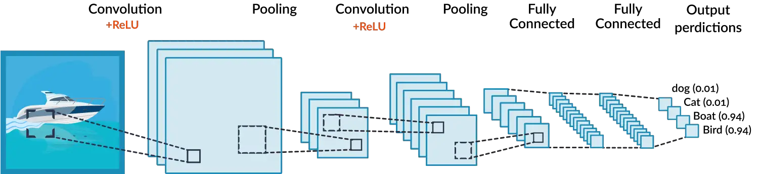
Keras provides many ready-to-use layer API and Keras convolution layer is just one of them. It is used for creating convolutions over an image in the CNN model.
Each convolution layer has some pre-defined properties in convolution neural networks. Let’s look at each of these properties and find out how they are used in Keras convolution layers.
- Filters − This helps in setting the number of filters that can be applied over a convolution. The count of filters also influences the dimension of the output shape.
- kernel size − This defines the length of the convolution window.
- Strides − We can set the stride length of convolution with this.
- Dilation Rate − Dilation rate determines how dilation is applied.
- data_format − This tells us about the kind of data present.
- Padding − Through this parameter, we can specify how padding operation will be performed. There are three options for this parameter −
-
-
- valid – means no padding
- causal – means causal convolution.
- same – means the output should have the same length as input and so, padding should be applied accordingly
-
The Keras library offers the below types of convolution layer –
- Conv 1-D Layer
- Conv 2-D Layer
- Conv-3D Layer
import tensorflow as tf
import keras
[adrotate banner=”3″]
Keras Conv-1D Layer
The Conv-1D Layer of Keras is used for creating the convolution kernel. It is generally convolved along with the input layer on the top of single spatial dimension used for producing a tensor of outputs. The use_bias parameter is created and added to outputs if it’s passed as true. If the activation is not passed as None then it’s added to output layer as well.
Syntax
tf.keras.layers.Conv1D(filters,kernel_size,strides=1,padding=”valid”,data_format=channels_last”,dilation_rate=1,groups=1,activation=None,use_bias=True, kernel_initializer=”glorot_uniform”,bias_initializer=”zeros”,kernel_regularizer=None,bias_regularizer=None,activity_regularizer=None,kernel_constraint=None,bias_constraint=None,kwargs)
Keras Conv-1D Layer Example
The below code snippet shows how a 1-D convolution layer is created. We’ll be able to see the shape obtained by output layer.
As we see the output layer shape is having length vectors reduced to 32 with only 10 timesteps.
 # The inputs are 128-length vectors with 12 timesteps, and the batch size is 5.
 input_shape = (5, 12, 128)
 x = tf.random.normal(input_shape)
 y = tf.keras.layers.Conv1D(32, 3, activation='relu',input_shape=input_shape[1:])(x)
 print(y.shape)
Keras Conv-2D Layer
Keras Conv-2D layer is the most widely used convolution layer which is helpful in creating spatial convolution over images.
This layer also follows the same rule as Conv-1D layer for using bias_vector and activation function.
Whenever we deal with images, we use this Conv-2D layer as it helps in reducing the size of images for faster processing.
Syntax
tf.keras.layers.Conv2D(filters,kernel_size,strides=(1,1), padding=”valid”, data_format=None,dilation_rate=(1, 1),groups=1,activation=None,use_bias=True,
kernel_initializer=”glorot_uniform”,bias_initializer=”zeros”,kernel_regularizer=None,bias_regularizer=None,activity_regularizer=None,kernel_constraint=None,bias_constraint=None,kwargs)
Keras Conv-2D Layer Example
Example – 1 : Simple Example of Keras Conv-2D Layer
This first example of conv-2D layer is consisting of 28×28 images and batch size of 4.
As we provide the input and add the convolution 2D layer. Lastly, the shape is displayed.
# The inputs are 28x28 RGB images with `channels_last` and the batch
# size is 4.
input_shape = (4, 28, 28, 3)
x = tf.random.normal(input_shape)
y = tf.keras.layers.Conv2D(2, 3, activation='relu', input_shape=input_shape[1:])(x)
print(y.shape)
Example – 2: Altering Dilation Rate in Keras Conv-2D Layer
In this second example, we are using the dilation rate parameter in Conv-2D.
Dilation is a technique used for creating a bigger image with more pixels that helps in image processing.
As we see in the output the image size has been reduced to 24×24 and also the batch size has become 2.
input_shape = (4, 28, 28, 3)
x = tf.random.normal(input_shape)
y = tf.keras.layers.Conv2D(2, 3, activation='relu', dilation_rate=2, input_shape=input_shape[1:])(x)
print(y.shape)
Example – 3 : Keeping Padding as ‘Same’ in Keras Conv-2D Layer
In this third example, we’ll be assigning the padding parameter value as “same”, as discussed before padding has three values.
The shape of the resulting layer is the same as the input layer but the batch size decreases.
input_shape = (4, 28, 28, 3)
x = tf.random.normal(input_shape)
y = tf.keras.layers.Conv2D(2, 3, activation='relu', padding="same", input_shape=input_shape[1:])(x)
print(y.shape)
Example – 4 : Extended Batch Shape [4, 7] in Keras Conv-2D Layer
This fourth example contains an extended batch shape for the input layer. When the Conv2D layer is applied to such inputs, we get the output layer with 26×26 images.
input_shape = (4, 7, 28, 28, 3)
x = tf.random.normal(input_shape)
y = tf.keras.layers.Conv2D(2, 3, activation='relu', input_shape=input_shape[2:])(x)
print(y.shape)
Keras Conv-3D Layer
The Conv-3D layer in Keras is generally used for operations that require 3D convolution layer (e.g. spatial convolution over volumes).
This layer creates a convolution kernel that is convolved with the layer input to produce a tensor of outputs. If use_bias is True, a bias vector is created and added to the outputs. Finally, if activation is not None, it is applied to the outputs as well.
Syntax
tf.keras.layers.Conv3D(filters,kernel_size,strides=(1, 1, 1),padding=”valid”, data_format=None, dilation_rate=(1, 1, 1), groups=1, activation=None, use_bias=True, kernel_initializer=”glorot_uniform”, bias_initializer=”zeros”, kernel_regularizer=None, bias_regularizer=None, activity_regularizer=None, kernel_constraint=None, bias_constraint=None, kwargs)
Example – 1 : Simple Example of Keras Conv-3D Layer
This first example of Conv-3D layer has a single channel or frame with 28x28x28 dimension. The input layer is supplied with random numbers in normalized form.
Next, a Keras Conv-3D layer is added to the input layer.
As we can see the shape of the output layer is altered as it contains 26x26x26 channel with batch size 2.
# The inputs are 28x28x28 volumes with a single channel, and the
# batch size is 1
input_shape =(4, 28, 28, 28, 1)
x = tf.random.normal(input_shape)
y = tf.keras.layers.Conv3D( 2, 3, activation='relu', input_shape=input_shape[1:])(x)
print(y.shape)
Example – 2 : Extended Batch Shape [4,7] in Keras Conv-3D Layer
The second example consists of an extended batch shape with 4 videos of 3D Frame where each video has 7 frames.
After applying the 3D convolutional layer we get 26x26x26 dimension results with batch size as 2.
# With extended batch shape [4, 7], e.g. a batch of 4 videos of 3D frames,
# with 7 frames per video.
input_shape = (4, 7, 28, 28, 28, 1)
x = tf.random.normal(input_shape)
y = tf.keras.layers.Conv3D( 2, 3, activation='relu', input_shape=input_shape[2:])(x)
print(y.shape)
Complete Example of Convolutional Neural Network with Keras Conv-2D Layer
Now in this section, we will be building a complete Convolutional Neural Network using the Keras library. This will be a 2D Convolutional Neural Network mainly used for image processing and finding insights from images.
Here the image dataset used is the MNIST dataset, which is an in-built dataset in the Keras library.
Loading Required Libraries
Here we are importing the required libraries such as numpy, matplotlib, scikit-learn for building models, and lastly Keras library that will also be used for loading the dataset for our model.
Different layers such as Sequential, Conv2D, Max Pooling 2D, Dense, SGD and Flatten are added.
# baseline cnn model for mnist
from numpy import mean
from numpy import std
from matplotlib import pyplot
from sklearn.model_selection import KFold
from keras.datasets import mnist
from keras.utils import to_categorical
from keras.models import Sequential
from keras.layers import Conv2D
from keras.layers import MaxPooling2D
from keras.layers import Dense
from keras.layers import Flatten
from keras.optimizers import SGD
Loading Dataset
The MNIST dataset is first loaded in the form of training and testing sets. The next step is the reshaping of the dataset to create a single channel.
Lastly, the training and testing sets are encoded for converting the target variable to the categorical data type.
The load_dataset() function returns training and testing datasets.
# load train and test dataset
def load_dataset():
	# load dataset
	(trainX, trainY), (testX, testY) = mnist.load_data()
	# reshape dataset to have a single channel
	trainX = trainX.reshape((trainX.shape[0], 28, 28, 1))
	testX = testX.reshape((testX.shape[0], 28, 28, 1))
	# one hot encode target values
	trainY = to_categorical(trainY)
	testY = to_categorical(testY)
	return trainX, trainY, testX, testY
Scaling Pixels
The next step after loading the dataset is to normalize the images present in the dataset.
First of all the datatype is altered from integers to float type. Next, the values are normalized so that all of them range between 0 to 1.
This function returns normalized images for both training and testing sets.
# scale pixels
def prep_pixels(train, test):
	# convert from integers to floats
	train_norm = train.astype('float32')
	test_norm = test.astype('float32')
	# normalize to range 0-1
	train_norm = train_norm / 255.0
	test_norm = test_norm / 255.0
	# return normalized images
	return train_norm, test_norm
Building CNN Model
As our data is ready, now we will be building the Convolutional Neural Network Model with the help of the Keras package.
The model is built with the help of Sequential API. The model is provided with a convolution 2D layer, then max pooling 2D layer is added along with flatten and two dense layers.
The next step while building a model is compiling it with the help of SGD i.e. stochastic gradient descent. The function returns a complete model.
# define cnn model
def define_model():
	model = Sequential()
	model.add(Conv2D(32, (3, 3), activation='relu', kernel_initializer='he_uniform', input_shape=(28, 28, 1)))
	model.add(MaxPooling2D((2, 2)))
	model.add(Flatten())
	model.add(Dense(100, activation='relu', kernel_initializer='he_uniform'))
	model.add(Dense(10, activation='softmax'))
	# compile model
	opt = SGD(lr=0.01, momentum=0.9)
	model.compile(optimizer=opt, loss='categorical_crossentropy', metrics=['accuracy'])
	return model
Evaluating the Model
Once a model is built, we need to evaluate our model for understanding its performance. In this example, we’ll be using k-fold cross validation method for this.
For the purpose of evaluation, the dataset is divided into three parts i.e. training data, testing data, and validation data.
The evaluate_model function will return the accuracy scores for the model and record of how the model fits the data.
# evaluate a model using k-fold cross-validation
def evaluate_model(dataX, dataY, n_folds=5):
	scores, histories = list(), list()
	# prepare cross validation
	kfold = KFold(n_folds, shuffle=True, random_state=1)
	# enumerate splits
	for train_ix, test_ix in kfold.split(dataX):
		# define model
		model = define_model()
		# select rows for train and test
		trainX, trainY, testX, testY = dataX[train_ix], dataY[train_ix], dataX[test_ix], dataY[test_ix]
		# fit model
		history = model.fit(trainX, trainY, epochs=10, batch_size=32, validation_data=(testX, testY), verbose=0)
		# evaluate model
		_, acc = model.evaluate(testX, testY, verbose=0)
		print('> %.3f' % (acc * 100.0))
		# stores scores
		scores.append(acc)
		histories.append(history)
	return scores, histories
Summarizing Diagnostic Learning Curves
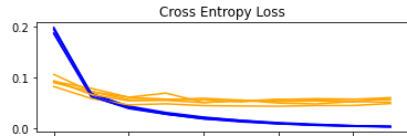
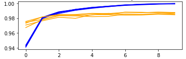
With the help of the below function, we are going to visualize the loss and accuracy obtained with the help of this model.
The plots will have information about both training datasets and testing datasets.
# plot diagnostic learning curves
def summarize_diagnostics(histories):
	for i in range(len(histories)):
		# plot loss
		pyplot.subplot(2, 1, 1)
		pyplot.title('Cross Entropy Loss')
		pyplot.plot(histories[i].history['loss'], color='blue', label='train')
		pyplot.plot(histories[i].history['val_loss'], color='orange', label='test')
		# plot accuracy
		pyplot.subplot(2, 1, 2)
		pyplot.title('Classification Accuracy')
		pyplot.plot(histories[i].history['accuracy'], color='blue', label='train')
		pyplot.plot(histories[i].history['val_accuracy'], color='orange', label='test')
	pyplot.show()
Visualizing Results
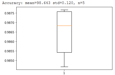
We will also visualize the accuracy with the help of a boxplot for a better understanding of results.
# summarize model performance
def summarize_performance(scores):
	# print summary
	print('Accuracy: mean=%.3f std=%.3f, n=%d' % (mean(scores)*100, std(scores)*100, len(scores)))
	# box and whisker plots of results
	pyplot.boxplot(scores)
	pyplot.show()
Execution
The run_test_harness() will help to invoke the above functions that we have already built.
In [16]:
# run the test harness for evaluating a model
def run_test_harness():
	# load dataset
	trainX, trainY, testX, testY = load_dataset()
	# prepare pixel data
	trainX, testX = prep_pixels(trainX, testX)
	# evaluate model
	scores, histories = evaluate_model(trainX, trainY)
	# learning curves
	summarize_diagnostics(histories)
	# summarize estimated performance
	summarize_performance(scores)
# entry point, run the test harness
run_test_harness()
Results
The final results show that the accuracy achieved by the model is around 98.75%.
The graphs of Cross-Entropy Loss and Classification Accuracy show that in the training set (depicted by the blue line) loss is almost 0% and accuracy is nearer to 100% whereas in the case of the testing set (depicted by the orange line) loss is nearer to 0.1% and accuracy is 98.75%.
The third graph i.e. boxplot actually shows the accuracy of the model, standard deviation, mean, data spread, and outliers.
Visualizing the result with Box Plot
- Also Read – Different Types of Keras Layers Explained for Beginners
- Also Read – Keras Dropout Layer Explained for Beginners
- Also Read – Keras Dense Layer Explained for Beginners
- Also Read – Keras vs Tensorflow vs Pytorch – No More Confusion !!
Conclusion
This article talked about different Keras convolution layers available for creating CNN models. We learned about Conv-1D Layer, Conv-2D Layer, and Conv-3D Layer in Keras and saw various examples about them. Finally, we also learned how we can implement a 2D convolutional neural network with the help of Keras libraries.
Reference Keras Documentation

