
Introduction
In this tutorial, we will explain the implementation of the Keras Dropout Layer. We will give a brief explanation of why the dropout layer is used in neural networks and then go through a detailed example of how to use the dropout layer in Keras. We will also understand the parameters that are used in the dropout layer function.
Why Dropout Layer is used?
Dropout Layer is one of the most popular regularization techniques to reduce overfitting in the deep learning models. Overfitting in the model occurs when it shows more accuracy on the training data but less accuracy on the test data or unseen data.
In the dropout technique, some of the neurons in hidden or visible layers are dropped or omitted randomly. The experiments show that this dropout technique regularizes the neural network model to produce a robust model which does not overfit.
Keras Dropout Layer Syntax and Parameters
Before we move on and look at the functioning of the dropout layer, let us look at the dropout function along with the parameters for better understanding of usage.
keras.layers.Dropout(rate, noise_shape = None, seed = None)
The parameters of the function are explained as follows:
- rate − This represents the fraction of the input unit to be dropped. It will be from 0 to 1.
- noise_shape – It represents the dimension of the shape in which the dropout to be applied. For example, the input shape is (batch_size, timesteps, features). Then, to apply dropout in the timesteps, (batch_size, 1, features) need to be specified as noise_shape
- seed − A Python integer is used as a random seed.
How to use Dropout Layer in Keras?
In this section, we’ll understand how to use the dropout layer with other layers of Keras.
- The dropout layer is actually applied per-layer in the neural networks and can be used with other Keras layers for fully connected layers, convolutional layers, recurrent layers, etc.
- Dropout Layer can be applied to the input layer and on any single or all the hidden layers but it cannot be applied to the output layer.
- The range of value for dropout is from 0 to 1. The higher the number, more input values will be dropped.
[adrotate banner=”3″]
Keras Dropout Layer Examples
Example – 1: Simple usage of Dropout Layers in Keras
The first example will just show the simple usage of Dropout Layers without building a big model.
Initially, data is generated, then the Dropout layer is added with the first parameter value i.e. “0.2” suggesting the number of values to be dropped.
The input data for the model is obtained using arange function. Then with this data, we perform the training of the model for obtaining the results.
import tensorflow as tf
import keras
import numpy as np

tf.random.set_seed(0)

layer = tf.keras.layers.Dropout(.2, input_shape=(2,))

data = np.arange(10).reshape(5, 2).astype(np.float32)

print(data)
The below cell shows how the output is obtained with the help of the added layer. After the layer is provided with the input data, training of the model is done, and then finally output is generated.
outputs = layer(data, training=True)
print(outputs)
Example – 2 : How Dropout Layer reduces overfitting in Neural Network
In this example, we will build two prediction models using Keras. In one model we’ll only use only dense layers and in another model, we will add the dropout layer. We will then compare the performance of these two models where the evaluation criteria will be the prediction result obtained on the test dataset.
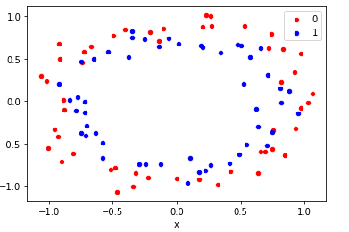
In this problem, we will generate random data samples with “make_circles” function of Keras and visualize it with a scatter plot using the Matplotlib library. Then we proceed to perform binary classification on the dataset with the model we build with Keras.
Generate Dataset
# generate two circles dataset
from sklearn.datasets import make_circles
from matplotlib import pyplot
from pandas import DataFrame
from sklearn import datasets

# generate 2d classification dataset
X, y = make_circles(n_samples=100, noise=0.1, random_state=1)
# scatter plot, dots colored by class value
df = DataFrame(dict(x=X[:,0], y=X[:,1], label=y))
colors = {0:'red', 1:'blue'}
fig, ax = pyplot.subplots()
grouped = df.groupby('label')
for key, group in grouped:
    group.plot(ax=ax, kind='scatter', x='x', y='y', label=key, color=colors[key])
pyplot.show()
Building a Model without Dropouts
The next step is to split the dataset into a training set and testing set. Now it’s time to create the model without a dropout layer.
X, y = make_circles(n_samples=100, noise=0.1, random_state=1)
# split into train and test
n_train = 30
trainX, testX = X[:n_train, :], X[n_train:, :]
trainy, testy = y[:n_train], y[n_train:]
Here Keras in-built models and layers are imported, we use Sequential model. After this, a couple of Dense layers are added, one with relu activation and the other one with sigmoid activation. Lastly, this model is compiled and we look to calculate the accuracy of the results with metrics parameter set to “accuracy”.
from keras import models
from keras import layers

# define model
model = models.Sequential()
model.add(layers.Dense(500, input_dim=2, activation='relu'))
model.add(layers.Dense(1, activation='sigmoid'))
model.compile(loss='binary_crossentropy', optimizer='adam', metrics=['accuracy'])
Now the above model is fitted and trained over the data available with us. Here we also specify the number of epochs(iterations).
# fit model
history = model.fit(trainX, trainy, validation_data=(testX, testy), epochs=4000, verbose=0)
At last, we will check the results of the model on testing data. The results will contains the accuracy value, thus suggesting how many values were correctly classified and how many weren’t classified correctly.
# evaluate the model
_, train_acc = model.evaluate(trainX, trainy, verbose=0)
_, test_acc = model.evaluate(testX, testy, verbose=0)
print('Train: %.3f, Test: %.3f' % (train_acc, test_acc))
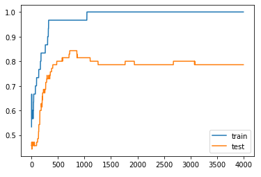
Clearly, the result shows that training accuracy is “1.000” which means 100% accuracy but we are not concerned with this value, the actual value to be looked at is the testing accuracy. It has resulted as “0.786” i.e. almost 79% accuracy.
With the help of the matplotlib library, we plot the testing and training accuracy values and clearly, it has overfitted.
# plot history
pyplot.plot(history.history['accuracy'], label='train')
pyplot.plot(history.history['val_accuracy'], label='test')
pyplot.legend()
pyplot.show()
Building a Model using Dropouts Layer
Now it’s time to use the Dropout layer in the model and see whether the performance will be boosted or not.
Again we’ll be using the same dataset, the model will now have another layer i.e. dropout layer. We have passed “0.5” in the Dropout function, this will actually drop 50% of input values for regularizing the dataset and the model as well.
# mlp with dropout on the two circles dataset
from sklearn.datasets import make_circles
from keras.models import Sequential
from keras.layers import Dense
from keras.layers import Dropout
from matplotlib import pyplot

# generate 2d classification dataset
X, y = make_circles(n_samples=100, noise=0.1, random_state=1)
# split into train and test
n_train = 30
trainX, testX = X[:n_train, :], X[n_train:, :]
trainy, testy = y[:n_train], y[n_train:]

# define model
model = Sequential()
model.add(Dense(500, input_dim=2, activation='relu'))
model.add(Dropout(0.4))
model.add(Dense(1, activation='sigmoid'))
model.compile(loss='binary_crossentropy', optimizer='adam', metrics=['accuracy'])

# fit model
history = model.fit(trainX, trainy, validation_data=(testX, testy), epochs=4000, verbose=0)

# evaluate the model
_, train_acc = model.evaluate(trainX, trainy, verbose=0)
_, test_acc = model.evaluate(testX, testy, verbose=0)
print('Train: %.3f, Test: %.3f' % (train_acc, test_acc))

# plot history
pyplot.plot(history.history['accuracy'], label='train')
pyplot.plot(history.history['val_accuracy'], label='test')
pyplot.legend()
pyplot.show()
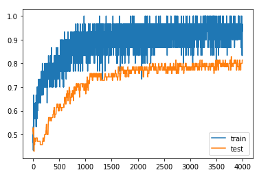
You can see for yourselves, there is a slight dip in training accuracy which is actually insignificant but the testing accuracy has increased. Testing Accuracy is “0.814” which means 81% and the is NO overfitting.
So this comparison-based example clearly shows that the dropout layer can boost the model performance and avoid overfitting.
Tips on using Dropout Layer
We will end this article by discussing some tips that one must remember while working with the Dropout layer.
- Experiments show that the dropout value should range from 20% to 50%. In case you choose values below this range then the desired effects won’t be visible and if the values above this range are chosen then the network may suffer from under-learning.
- If the resources permit, try to use a larger network as this has more probability of giving better results. This is also because the model will get more opportunities to learn.
- Remember that the dropout layer can be used on all the visible i.e. input units and also on hidden units. Results have been pretty good if dropout is used at each layer of a network.
Conclusion
The tutorial explained the Keras DropoutLlayer function and its parameters, where we discussed the importance of the dropout layer. We also covered examples to show how dropout can reduce overfitting.
Reference Keras Documentation

