
What is Decision Tree?
Decision tree is a type of supervised learning algorithm that can be used for both regression and classification problems. The algorithm uses training data to create rules that can be represented by a tree structure.
Like any other tree representation, it has a root node, internal nodes, and leaf nodes. The internal node represents condition on attributes, the branches represent the results of the condition and the leaf node represents the class label.
Making of Decision Tree
For making a decision tree, at each level we have to make a selection of the attributes to be the root node. This is known as attributes selection. This is mainly done using :
- Gini index.
- Information gain.
- chi-square.
Advantages of Decision Tree
There are some advantages of using a decision tree as listed below –
- The decision tree is a white-box model. We can easily understand any particular condition of the model which results in either true or false.
- It can handle both continuous and categorical data.
Disadvantages of Decision Tree
- Decision trees may become very large and complex with a large number of attributes.
- A decision tree at times can be sensitive to the training data, a very small variation in data can lead to a completely different tree structure.
Applications of Decision Tree
Some of the real-world and practical applications of decision tree are –
- Loan Application Approval
- Prediction of Customer Churn
- Fraud Detection
- Medical Diagnosis
Example of Decision Tree Classifier in Python Sklearn
Scikit Learn library has a module function DecisionTreeClassifier() for implementing decision tree classifier quite easily.
We will show the example of the decision tree classifier in Sklearn by using the Balance-Scale dataset. The goal of this problem is to predict whether the balance scale will tilt to the left or right based on the weights on the two sides.
The data can be downloaded from the UCI website by using this link
Importing Libraries
We will start by importing the initial required libraries such as NumPy, pandas, seaborn, and matplotlib.pyplot. The Sklearn modules will be imported in the later section.
import numpy as np
import pandas as pd
import seaborn as sns
import matplotlib.pyplot as plt
%matplotlib inline
Importing Dataset
Next, we import the dataset from the CSV file to the Pandas dataframes.
col = [ 'Class Name','Left weight','Left distance','Right weight','Right distance']
df = pd.read_csv('balance-scale.data',names=col,sep=',')
df.head()
Information About Dataset
We can get the overall information of our data set by using the df.info function. From the output, we can see that it has 625 records with 5 fields.
df.info()
Exploratory Data Analysis (EDA)
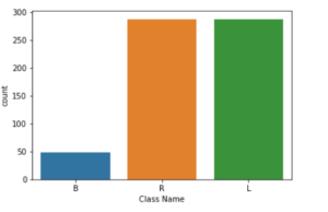
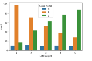
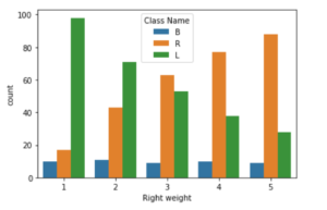
Let us do a bit of exploratory data analysis to understand our dataset better. We have plotted the classes by using countplot function. We can see in the figure given below that most of the classes names fall under the labels R and L which means Right and Left respectively. Very few data fall under B, which stands for balanced.
sns.countplot(df['Class Name'])
sns.countplot(df['Left weight'],hue=df['Class Name'])
sns.countplot(df['Right weight'],hue=df['Class Name'])
Splitting the Dataset in Train-Test
Before feeding the data into the model we first split it into train and test data using the train_test_split function.
from sklearn.model_selection import train_test_split
X = df.drop('Class Name',axis=1)
y = df[['Class Name']]
X_train, X_test, y_train, y_test = train_test_split(X, y, test_size = 0.3,random_state=42)
Training the Decision Tree Classifier
We have used the Gini index as our attribute selection method for the training of decision tree classifier with Sklearn function DecisionTreeClassifier().
We have created the decision tree classifier by passing other parameters such as random state, max_depth, and min_sample_leaf to DecisionTreeClassifier().
Finally, we do the training process by using the model.fit() method.
from sklearn.tree import DecisionTreeClassifier
clf_model = DecisionTreeClassifier(criterion="gini", random_state=42,max_depth=3, min_samples_leaf=5)
clf_model.fit(X_train,y_train)
Test Accuracy
We will now test accuracy by using the classifier on test data. For this we first use the model.predict function and pass X_test as attributes.
y_predict = clf_model.predict(X_test)
Next, we use accuracy_score function of Sklearn to calculate the accuracty. We can see that we are getting a pretty good accuracy of 78.6% on our test data.
from sklearn.metrics import accuracy_score,classification_report,confusion_matrix
accuracy_score(y_test,y_predict)
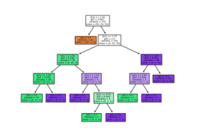
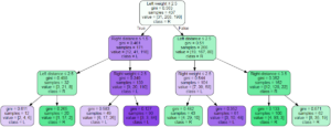
Plotting Decision Tree
We can plot our decision tree with the help of the Graphviz library and passing after a bunch of parameters such as classifier model, target values, and the features name of our data.
target = list(df['Class Name'].unique())
feature_names = list(X.columns)
from sklearn import tree
import graphviz
dot_data = tree.export_graphviz(clf_model,
                                out_file=None,
                      feature_names=feature_names,
                      class_names=target,
                      filled=True, rounded=True,
                      special_characters=True)
graph = graphviz.Source(dot_data)

graph

We can also get a textual representation of the tree by using the export_tree function from the Sklearn library
from sklearn.tree import export_text
r = export_text(clf_model, feature_names=feature_names)
print(r)
We can save the graph using the save() method.
graph.save('graph1.jpg')
- Also Read – Linear Regression in Python Sklearn with Example
- Also Read – Python Sklearn Logistic Regression Tutorial with Example
Conclusion
Hope you liked our tutorial and now understand how to implement decision tree classifier with Sklearn (Scikit Learn) in Python. We showed you an end-to-end example using a dataset to build a decision tree model for the predictive task using SKlearn DecisionTreeClassifier() function.


2 Responses
Hi, great tutorial but I have one question! If you already have two separate CSV files for train and test data, how would that work here?
Thanks!
In that case you may avoid splitting of dataset and use the train & test csv files to load and assign them to X_Train and X_Test respectively.