Introduction
In this article, we will see a tutorial on Random Forest Regression by using Python Sklearn library. We will have a brief overview of Random Forest Regression and then understand the RandomForestRegressor module of Sklearn in detail. Finally, we will see its example with the help of a small machine learning project that will also include hyperparameter tuning for RandomForestRegressor.
Quick Overview on Random Forest Regression
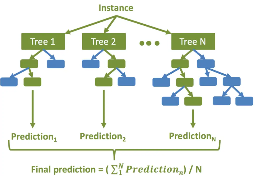
Random Forest is an ensemble learning technique used for both classification and regression problems. In this technique, multiple decision trees are created and their output is averaged to give the final result. Random Forest Regression is known to produce very robust results by avoiding overfitting.
How Random Forest Regression Works
The high-level steps for random forest regression are as followings –
- Decide the number of decision trees N to be created.
- Randomly take K data samples from the training set by using the bootstrapping method.
- Create a decision tree using the above K data samples.
- Repeat steps 2 and 3 till N decision trees are created.
- For the new unseen data predict regression results using each of the N decision trees. Then take an average of these results to arrive at the final regression output.
Random Forest Regression in Sklearn
In Sklearn, random forest regression can be done quite easily by using RandomForestRegressor module of sklearn.ensemble module.
Random Forest Regressor Hyperparameters (Sklearn)
Hyperparameters are those parameters that can be fine-tuned for arriving at better accuracy of the machine learning model. Some of the main hyperparameters that RandomForestRegressor module of Sklearn provides are as follows –
- n_estimators: It denotes the number of decision trees to be created in the random forest model. By default, it is 100.
- criterion: This denotes the criteria to be used to assess the quality of the split in decision trees. The supported values are ‘squared_error’ (default), ‘absolute_error’, ‘friedman_mse’, ‘poisson’.
- max_depth: It denotes the maximum depth of the tree. By default is None in which case nodes are expanded till all leaves become pure or until all leaves contain less than min_samples_split samples.
- min_samples_split: It denotes the minimum number of samples needed to split an internal node. By default, it is 2.
- min_samples_leaf: It denotes the minimum number of samples required to be at the leaf node. By default, it is 1.
- max_features: It denotes the number of features to be considered for the best split. It can have values of ‘auto’, ‘sqrt’, ‘log2’, ‘None’, int, or float value. By default, it is 1.0
- max_samples: It denotes the number of samples to be drawn from training data in bootstrap sampling.
Example of Random Forest Regression in Sklearn
About Dataset
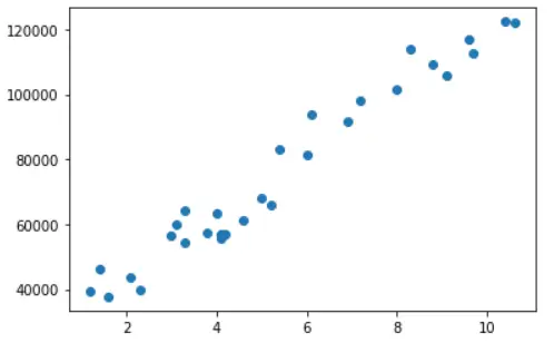
In this example, we are going to use the Salary dataset which contains two attributes – ‘YearsExperience’ and ‘Salary’. It is a simple and small dataset of only 29 records.
Importing libraries
To begin with, we import all the libraries that are going to be required in this example including RandomForestRegressor.
In [0]:
import numpy as np
import pandas as pd
import matplotlib.pyplot as plt

from sklearn.model_selection import train_test_split
from sklearn.metrics import r2_score
from sklearn.model_selection import GridSearchCV

from sklearn.ensemble import RandomForestRegressor
Importing Dataset
Next, we import the dataset into Pandas DataFrame and list down its row.
In [1]:
df = pd.read_csv('/content/salary_dataset.csv')

df
| index | YearsExperience | Salary |
|---|---|---|
| 0 | 1.2 | 39344 |
| 1 | 1.4 | 46206 |
| 2 | 1.6 | 37732 |
| 3 | 2.1 | 43526 |
| 4 | 2.3 | 39892 |
| 5 | 3.0 | 56643 |
| 6 | 3.1 | 60151 |
| 7 | 3.3 | 54446 |
| 8 | 3.3 | 64446 |
| 9 | 3.8 | 57190 |
| 10 | 4.0 | 63219 |
| 11 | 4.1 | 55795 |
| 12 | 4.1 | 56958 |
| 13 | 4.2 | 57082 |
| 14 | 4.6 | 61112 |
| 15 | 5.0 | 67939 |
| 16 | 5.2 | 66030 |
| 17 | 5.4 | 83089 |
| 18 | 6.0 | 81364 |
| 19 | 6.1 | 93941 |
| 20 | 6.9 | 91739 |
| 21 | 7.2 | 98274 |
| 22 | 8.0 | 101303 |
| 23 | 8.3 | 113813 |
| 24 | 8.8 | 109432 |
| 25 | 9.1 | 105583 |
| 26 | 9.6 | 116970 |
| 27 | 9.7 | 112636 |
| 28 | 10.4 | 122392 |
| 29 | 10.6 | 121873 |
Visualizing Dataset
Let us visualize the dataset by creating a scatter plot of matplotlib library.
In [2]:
plt.scatter(x = df['YearsExperience'], y = df['Salary'])
Out[2]:
Splitting the Dataset into Train & Test Dataset
In this section, we are first creating a dataframe of independent variable X and dependent variable y from the original dataframe df. Then we use train_test_split module to randomly create train and test datasets with an 80-20% split.
In [3]:
X = df.iloc[:, :-1]
y = df.iloc[:, -1]

X_train, X_test, y_train, y_test = train_test_split(X, y, test_size = 0.2, random_state = 0)
Training the RandomForestRegressor
Now we are creating an object of RandomForestRegressor with n_estimators = 10 i.e. with 10 decision trees. And then we fit this object over X_train and y_train for training the model.
In [4]:
rf_regressor = RandomForestRegressor(n_estimators = 10, random_state = 0)
rf_regressor.fit(X_train, y_train)
Training Accuracy
y_pred_train = rf_regressor.predict(X_train)
r2_score(y_train, y_pred_train)
0.9815329041236582
Visualizing Training Accuracy
fig, ax = plt.subplots()
ax.scatter(X_train,y_train, color = "red")
ax.scatter(X_train,y_pred_train, color = "blue")
Out[6]:
Testing Accuracy
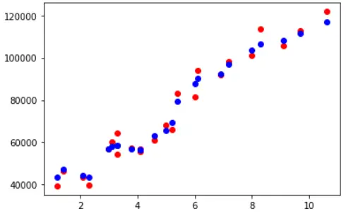
Now we use this model to carry out predictions on unseen test data and check its accuracy which turns out to be 96.7%. This indicates, there is slight overfitting in the model because its training accuracy was 98.1%. We shall address this in the next section of hyperparameter tuning.
In[7]:
y_pred = rf_regressor.predict(X_test)
r2_score(y_test, y_pred)
0.9675706804534532
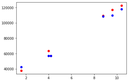
Visualizing Testing Accuracy
Again, let us visualize the testing accuracy with the help of matplotlib scatter plot. The red markers are actual data points and the blue ones are corresponding predicted data points.
In [8]:
fig, ax = plt.subplots()
ax.scatter(X_test,y_test, color = "red")
ax.scatter(X_test,y_pred, color = "blue")
Improving Results with K Cross Validation & Hyperparameter Tuning
In the above example, we noticed slight overfitting in the trained model. This is because the dataset is very small (29 rows) and splitting it into train and test sets can lead to information loss for training. Thus an effective way is to use K Cross Validation instead of splitting the data to produce a good model less prone to overfitting.
Secondly, in the example, we just use n_estimators as 10 but we can also play around with different combinations and values of other hyperparameters. We cannot evaluate so many combinations manually, hence we can use GridSearchCV module of Sklearn.
- Also Read – Cross Validation in Sklearn
- Also Read – Hyperparameter Tuning with Sklearn GridSearchCV
Let us see the implementation below.
Using GridSearchCV & Cross Validation
Here we first create param_grid with multiple hyperparameters and their possible values using which we want to create & evaluate the model. We then use this param_grid, the RandomForestRegressor object to create an instance of GridSearchCV with K Cross Validation value cv=5 & scoring technique as R2.
Finally, we fit the GridSearchCV object over the training dataset. During this process, GridSearchCV creates different models with all possible combinations of hyperparameters that we provided in param_grid.
In [9]:
param_grid = {
    'bootstrap': [True],
    'max_depth': [80, 90, 100, None],
    'max_features': ["sqrt", "log2", None],
    'min_samples_leaf': [1, 3, 5],
    'min_samples_split': [2, 3, 4],
    'n_estimators': [10, 25, 50, 75, 100]
}

rf = RandomForestRegressor()
grid_search = GridSearchCV(estimator = rf, param_grid = param_grid, cv = 5, verbose =2, scoring='r2',  n_jobs = -1)
grid_search.fit(X_train, y_train)
Fitting 5 folds for each of 540 candidates, totalling 2700 fits
GridSearchCV(cv=5, estimator=RandomForestRegressor(), n_jobs=-1,
             param_grid={'bootstrap': [True], 'max_depth': [80, 90, 100, None],
                         'max_features': ['sqrt', 'log2', None],
                         'min_samples_leaf': [1, 3, 5],
                         'min_samples_split': [2, 3, 4],
                         'n_estimators': [10, 25, 50, 75, 100]},
             scoring='r2', verbose=2)
Checking for Best Hyperparameters
Let us see the best hyperparameter combination that GridSearchCV has selected for us.
In [10]:
grid_search.best_params_
{'bootstrap': True,
 'max_depth': None,
 'max_features': None,
 'min_samples_leaf': 1,
 'min_samples_split': 3,
 'n_estimators': 25}
Training Accuracy
The training accuracy here comes out to be 98.4%
In [11]:
y_pred = best_grid.predict(X_train)
r2_score(y_train, y_pred)
Out[11]:
0.9846484854275217
Testing Accuracy
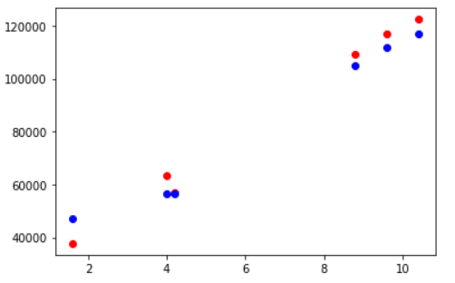
The accuracy on the unseen test data comes out to be 97.9% ~ 98% which is equivalent to the accuracy we got on training data. This means by using K Cross Validation and hyperparameter tuning with GridSearchCV we are able to avoid overfitting.
In [12]:
y_pred = best_grid.predict(X_test)
r2_score(y_test, y_pred)
Out[12]:
0.9792332560698718
Visualizing Testing Accuracy
In this visualization, we can see that the red and blue markers that correspond to actual and predicted data are much closer than what we saw in the earlier example. Hence this confirms that we have achieved better accuracy with K Cross Validation and GridSearchCV.
In [13]:
fig, ax = plt.subplots()
ax.scatter(X_test,y_test, color = "red")
ax.scatter(X_test,y_pred, color = "blue")
Reference: Sklearn Documentation