Introduction
In this tutorial, we will learn and implement an unsupervised learning algorithm of DBSCAN Clustering in Python Sklearn. First, we will briefly understand how the DBSCAN algorithm works along with some key concepts of epsilon (eps), minPts, types of points, etc. Then we will cover an example for DBSCAN in Sklearn where we will also see how to find the optimum value of epsilon for creating good clusters.
1. What is DBSCAN Clustering Algorithm
DBSCAN stands for Density-Based Spatial Clustering of Applications with Noise. It belongs to the unsupervised learning family of clustering algorithms.
When it comes to clustering, usually K-means or Hierarchical clustering algorithms are more popular. But they work well only when the clusters are simple to detect. They will not produce good results when the clusters have complex shapes or structures and this is where the DBSCAN algorithm gets the upper hand.
DBSCAN is a density-based clustering algorithm that assumes that clusters are dense regions in space that are separated by regions having a lower density of data points. Here, the ‘densely grouped’ data points are combined into one cluster. We can identify clusters in large datasets by observing the local density of data points.
A unique feature of DBSCAN clustering is that it is robust to outliers, due to which it finds an application in anomaly detection systems. In addition to that, it does not require the number of clusters to be fed as input, unlike K-Means, where we have to manually specify the number of centroids.
Key Characteristics of DBSCAN Algorithm
- It does not require the number of clusters as input.
- It is can detect outliers while finding clusters.
- DBSCAN algorithm can detect clusters that are complex or randomly shaped and sized.
2. Pre-requisite Concepts for DBSCAN
i) Epsilon Value (eps)
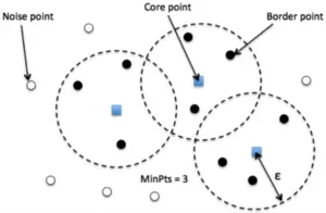
Epsilon is the radius of the circle around a data point such that all other data points that fall inside the circle are considered as neighborhood points. In other words, two points are considered to be neighbors if the distance between them is less than or equal to eps.
If the eps value is extremely small, then most of the points may not lie in the neighborhood and will be treated as outliers. This will result in bad clustering as most of the points fail to satisfy the minimum no. of points required to create a dense region.
On the other hand, if an extremely high value is chosen, then the majority of data points will remain in the same cluster. This will again create bad clustering where multiple clusters may end up merging due to the high value of epsilon.
Ideally, we must choose the eps value based on the distance of the dataset (using k-distance graph), however, normally small eps values are preferred.
ii) Minimum Points minPts
In DBSCAN minPts is the minimum number of data points that should be there in the region to define the cluster. You can choose the value of minPts based on your domain knowledge. But if you lack domain knowledge a good reference point is to have minPts ≥ D + 1 where D is the dimension of the dataset.
It is recommended to keep the value for the minPts at least 3, but for larger data sets, a greater minPts value should be chosen, especially if it has many outliers.
iii) Types of Points in DBSCAN Clustering
Based on the above two parameters, a point can be classified as:
- Core point: A core point is one in which at least have minPts number of points (including the point itself) in its surrounding region within the radius eps.
- Border point: A border point is one in which is reachable from a core point and there are less than minPts number of points within its surrounding region.
- Outlier: An outlier is neither a core point and nor is it reachable from any core points.
3. DBSCAN Clustering Algorithm
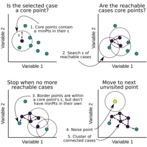
We start with the data points and values of epsilon and minPts as input –
- We select a random starting point that has not been visited.
- Determine the neighborhood of this point using epsilon which essentially acts as a radius.
- If the points in the neighborhood satisfy minPts criteria then the point is marked as a core point. The clustering process will start and the point is marked as visited else this point is labeled as noise.
- All points within the neighborhood of the core point are also marked as part of the cluster and the above procedure from step 2 is repeated for all epsilon neighborhood points.
- A new unvisited point is fetched, and following the above steps they are either included to form another cluster or they are marked as noise.
- The above process is continued till all points are visited.
4. Example of DBSCAN Clustering in Python Sklearn
The DBSCAN clustering in Sklearn can be implemented with ease by using DBSCAN() function of sklearn.cluster module. We will use a built-in function make_moons() of Sklearn to generate a dataset for our DBSCAN example as explained in the next section.
Import Libraries
To begin with, the required sklearn libraries are imported as shown below.
import pandas as pd
import numpy as np
from sklearn.datasets import make_moons
import matplotlib.pyplot as plt
import seaborn as sns
from sklearn.cluster import DBSCAN
from sklearn.metrics import silhouette_score
from sklearn.metrics import v_measure_score
The Dataset
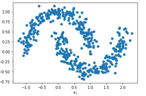
The make_moons() function is used in binary classification and generates a swirl pattern that looks like two moons. The noise factor for generating moon shape and the number of samples can be controlled with the help of parameters.
This generated pattern can be used as a dataset for our DBSCAN clustering example. In the illustration below we generate a moon dataset with moderate noise.
Below, we generate a sample of 500 data points with make_moons() with noise = 0.1 and then use this to create a pandas DataFrame to have a look at two columns X1 and X2.
X, y = make_moons(n_samples=500, noise=0.1)
df=pd.DataFrame(X,y)
df=df.rename(columns={0: "X1", 1:"X2"})
df.head()
| X1 | X2 | |
|---|---|---|
| 1 | 2.032188 | 0.100502 |
| 0 | -0.976073 | 0.316752 |
| 1 | 2.029438 | 0.316930 |
| 0 | -0.931001 | 0.036861 |
| 0 | -0.371835 | 0.989145 |
plt.scatter(X[:, 0], X[:, 1], c=y, label=y)
plt.xlabel("$x_1$")
plt.ylabel("$x_2$")
Text(0, 0.5, '$x_2$')
Applying Sklearn DBSCAN Clustering with default parameters
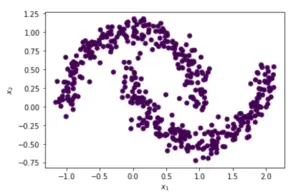
In this example, by using the default parameters of the Sklearn DBSCAN clustering function, our algorithm is unable to find distinct clusters and hence a single cluster with zero noise points is returned.
We need to fine-tune these parameters to create distinct clusters.
dbscan_cluster1 = DBSCAN()
dbscan_cluster1.fit(X)

# Visualizing DBSCAN
plt.scatter(X[:, 0],
            X[:, 1],
            c=dbscan_cluster1.labels_,
            label=y)
plt.xlabel("$x_1$")
plt.ylabel("$x_2$")

# Number of Clusters
labels=dbscan_cluster1.labels_
N_clus=len(set(labels))-(1 if -1 in labels else 0)
print('Estimated no. of clusters: %d' % N_clus)

# Identify Noise
n_noise = list(dbscan_cluster1.labels_).count(-1)
print('Estimated no. of noise points: %d' % n_noise)

# Calculating v_measure
print('v_measure =', v_measure_score(y, labels))
Estimated no. of clusters: 1
Estimated no. of noise points: 0
v_measure = 0.0
Applying DBSCAN with eps = 0.1 and min_samples = 8
dbscan_cluster = DBSCAN(eps=0.1, min_samples=8)
dbscan_cluster.fit(X)

# Visualizing DBSCAN
plt.scatter(X[:, 0],
X[:, 1],
c=dbscan_cluster.labels_,
label=y)
plt.xlabel("$x_1$")
plt.ylabel("$x_2$")

# Number of Clusters
labels=dbscan_cluster.labels_
N_clus=len(set(labels))-(1 if -1 in labels else 0)
print('Estimated no. of clusters: %d' % N_clus)

# Identify Noise
n_noise = list(dbscan_cluster.labels_).count(-1)
print('Estimated no. of noise points: %d' % n_noise)

# Calculating v_measure
print('v_measure =', v_measure_score(y, labels))
Out[7]:
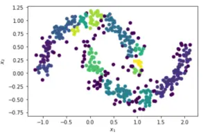
Estimated no. of clusters: 14
Estimated no. of noise points: 88
v_measure = 0.353411158836534
Finding the Optimal value of Epsilon
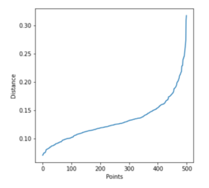
Rather than experimenting with different values of epsilon, we can use the elbow point detection method to arrive at a suitable value of epsilon.
In this approach, the average distance between each point and its k nearest neighbors is calculated where k = the MinPts selected by us. We then plot the average k-distances in ascending order on a k-distance graph
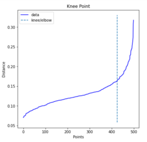
The optimal value for epsilon is the point with maximum curvature or bend, i.e. at the greatest slope.
Let us implement this technique below and generate a graph.
from sklearn.neighbors import NearestNeighbors

nearest_neighbors = NearestNeighbors(n_neighbors=11)
neighbors = nearest_neighbors.fit(df)

distances, indices = neighbors.kneighbors(df)
distances = np.sort(distances[:,10], axis=0)

fig = plt.figure(figsize=(5, 5))
plt.plot(distances)
plt.xlabel("Points")
plt.ylabel("Distance")
Text(0, 0.5, 'Distance')
Identifying Elbow Point with Kneed Package
from kneed import KneeLocator

i = np.arange(len(distances))
knee = KneeLocator(i, distances, S=1, curve='convex', direction='increasing', interp_method='polynomial')

fig = plt.figure(figsize=(5, 5))
knee.plot_knee()
plt.xlabel("Points")
plt.ylabel("Distance")

print(distances[knee.knee])
0.16354673748319307
<Figure size 360x360 with 0 Axes>
Applying DBSCAN with Optimal value of Epsilon = 0.163
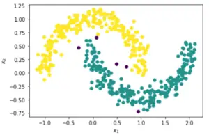
Now that we have derived the optimal value of epsilon as 0.163 above, let us use this in the DBSCAN algorithm below.
This time it is quite evident that the DBSCAN clustering is done properly with two resulting clusters and only 5 noise points. Even the v_measure_score is good with a value of 0.89
dbscan_cluster = DBSCAN(eps=0.163, min_samples=8)
dbscan_cluster.fit(X)

# Visualizing DBSCAN
plt.scatter(X[:, 0],
X[:, 1],
c=dbscan_cluster.labels_,
label=y)
plt.xlabel("$x_1$")
plt.ylabel("$x_2$")

# Number of Clusters
labels=dbscan_cluster.labels_
N_clus=len(set(labels))-(1 if -1 in labels else 0)
print('Estimated no. of clusters: %d' % N_clus)

# Identify Noise
n_noise = list(dbscan_cluster.labels_).count(-1)
print('Estimated no. of noise points: %d' % n_noise)

# Calculating v_measure
print('v_measure =', v_measure_score(y, labels))
Estimated no. of clusters: 2
Estimated no. of noise points: 5
v_measure = 0.8907602346423256
Conclusion
We hope you liked our tutorial and now better understand how to implement the DBSCAN clustering in Sklearn. Here, we have illustrated an end-to-end example of using a dataset to perform clustering and also explained to you that how to find the optimal value of epsilon for best clustering results.
References:
- https://iopscience.iop.org/article/10.1088/1755-1315/31/1/012012/pdf
- https://scikit-learn.org/stable/modules/generated/sklearn.cluster.DBSCAN.html
- https://www.kdnuggets.com/2020/04/dbscan-clustering-algorithm-machine-learning.html
- https://www.geeksforgeeks.org/ml-v-measure-for-evaluating-clustering-performance/
- https://sites.google.com/site/dataclusteringalgorithms/density-based-clustering-algorithm
-
I am passionate about Analytics and I am looking for opportunities to hone my current skills to gain prominence in the field of Data Science.
View all posts



2 Responses
Thanks, this helped a lot
Thank You for the feedback.