Introduction
In this article, we will look at a Decision Tree Regression tutorial using the Python Sklearn library. We will begin with a brief overview of Decision Tree Regression before going in-depth into Sklearn’s DecisionTreeRegressor module. Finally, we will see an example of it using a small machine learning project that will also include DecisionTreeRegressor hyperparameter tuning.
Quick Overview of Decision Tree Regression
How Decision Tree Regression Works – Step By Step
- Data Collection: The first step in creating a decision tree regression model is to collect a dataset containing both input features (also known as predictors) and output values (also called target variable).
- Test Train Data Splitting: The dataset is then divided into two parts: a training set and a testing set. The model is built using the training set, and its performance is evaluated using the testing set.
- Building Decision Tree: The decision tree is constructed by recursively splitting the training set into smaller subsets. The goal is to create a tree with high predictive accuracy while remaining simple to understand.
- Choosing the Best Split: At each stage of the tree-building process, the algorithm chooses the feature that best divides the data into the most homogeneous subsets based on a predefined criterion, such as mean squared error.
- Pruning the Tree: Once the tree is fully grown, it is often pruned to reduce overfitting. Pruning involves removing branches of the tree that do not improve the predictive accuracy of the model.
- Making Predictions: Predictions are made by passing the input data down the tree, traversing the branches until it reaches a leaf node. The leaf node’s output value is then used as a prediction for the input data.
- Evaluating the Model: The model’s performance is evaluated using the testing set. The model’s evaluation metric is chosen by the problem at hand, but it could be mean squared error, mean absolute error, R-squared, R Score, etc.
- Using the Model: Once trained and evaluated, the model can be used to make predictions on new, previously unseen data.
Decision Tree Regression in Sklearn
In Sklearn, decision tree regression can be done quite easily by using DecisionTreeRegressor module of sklearn.tree package.
Decision Tree Regressor Hyperparameters (Sklearn)
Hyperparameters are parameters that can be fine-tuned to improve the accuracy of a machine learning model. Some of the main hyperparameters provided by Sklearn’s DecisionTreeRegressor module are as follows:
criterion: This refers to the criteria that is used to evaluate the quality of the split in decision trees. The following values are supported:’squared error’ (the default), ‘absolute error’, ‘friedman mse’, and ‘poisson’.
splitter: This denotes the strategy used for splitting at each node while creating the tree. The supported strategies are “best” (default) and “random”.
max_depth: It denotes the tree’s maximum depth. It supports any int value or “None”. If “None”, nodes are expanded until all leaves are pure or contain fewer than min samples split samples.
min_samples_split: It refers to the minimum number of samples needed to split an internal node. It supports any int or float value and the default is 2.
min_samples_leaf: It refers to the minimum no. of samples required at the leaf node. By default, it is 1. It can be any int or float value and the default is 1.
max_features: It indicates the number of features to be considered in order to find the best split. It can have the values ‘auto,”sqrt,’ ‘log2’, ‘None,’ int, or float. It is set to 1.0 by default.
Example of Decision Tree Regression in Sklearn
About Dataset
In this example, we’ll use the Salary dataset, which has two attributes: ‘YearsExperience’ and ‘Salary’. It is a simple dataset with only 29 records.
Importing libraries
To begin, we import all of the libraries that will be needed in this example, including DecisionTreeRegressor.
In [0]:
import numpy as np
import pandas as pd
import matplotlib.pyplot as plt

from sklearn.model_selection import train_test_split
from sklearn.metrics import r2_score
from sklearn.model_selection import GridSearchCV

from sklearn.tree import DecisionTreeRegressor
Importing Dataset
Next, our dataset is imported into Pandas DataFrame and its rows are listed.
In [1]:
df = pd.read_csv('/content/salary_dataset.csv')

df
| index | YearsExperience | Salary |
|---|---|---|
| 0 | 1.2 | 39344 |
| 1 | 1.4 | 46206 |
| 2 | 1.6 | 37732 |
| 3 | 2.1 | 43526 |
| 4 | 2.3 | 39892 |
| 5 | 3.0 | 56643 |
| 6 | 3.1 | 60151 |
| 7 | 3.3 | 54446 |
| 8 | 3.3 | 64446 |
| 9 | 3.8 | 57190 |
| 10 | 4.0 | 63219 |
| 11 | 4.1 | 55795 |
| 12 | 4.1 | 56958 |
| 13 | 4.2 | 57082 |
| 14 | 4.6 | 61112 |
| 15 | 5.0 | 67939 |
| 16 | 5.2 | 66030 |
| 17 | 5.4 | 83089 |
| 18 | 6.0 | 81364 |
| 19 | 6.1 | 93941 |
| 20 | 6.9 | 91739 |
| 21 | 7.2 | 98274 |
| 22 | 8.0 | 101303 |
| 23 | 8.3 | 113813 |
| 24 | 8.8 | 109432 |
| 25 | 9.1 | 105583 |
| 26 | 9.6 | 116970 |
| 27 | 9.7 | 112636 |
| 28 | 10.4 | 122392 |
| 29 | 10.6 | 121873 |
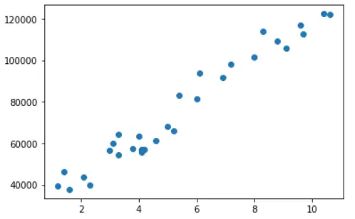
Visualizing Dataset
Let’s visualize the dataset using the Matplotlib library’s scatter plot.
In [2]:
plt.scatter(x = df['YearsExperience'], y = df['Salary'])
Out[2]:
Splitting the Dataset into Train & Test Dataset
In this section, we first divide the original data frame df into two data frames with independent variable X and dependent variable y. Then, we randomly generate train and test datasets with an 80-20% split using the train test split package. Moreover, the random state is kept at 5 to maintain the same split between reruns.
In [3]:
X = df.iloc[:, :-1]
y = df.iloc[:, -1]

X_train, X_test, y_train, y_test = train_test_split(X, y, test_size = 0.2, random_state = 4)
Training the DecisionTreeRegressor
Now we will create an object of DecisionTreeRegressor with random_state=0 so that the results can be reproduced in multiple reruns. And then we fit this regressor object over X_train and y_train for training the model.
In [4]:
dt_regressor = DecisionTreeRegressor(random_state = 0)
dt_regressor.fit(X_train, y_train)
Training Accuracy
y_pred_train = dt_regressor.predict(X_train)
r2_score(y_train, y_pred_train)
0.9971006453393606
Visualizing Training Accuracy
fig, ax = plt.subplots()
ax.scatter(X_train,y_train, color = "red")
ax.scatter(X_train,y_pred_train, color = "blue")
Out[6]:
Testing Accuracy
Now we utilize this model to carry out predictions on unseen test data and check its accuracy which turns out to be 98.8%. This indicates, there is slight overfitting in the model because its training accuracy was 99.7%. This issue will be covered in the following section on hyperparameter tuning of decision tree regression.
In [7]:
y_pred = dt_regressor.predict(X_test)
r2_score(y_test, y_pred)
0.9887060585499007
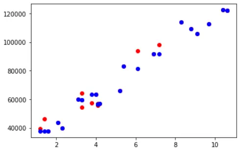
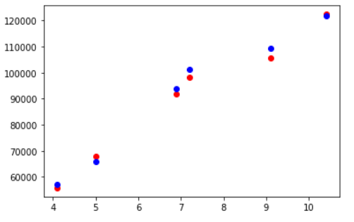
Visualizing Testing Accuracy
Again, let’s use a matplotlib scatter plot to illustrate the testing accuracy. The blue markers represent the appropriate projected data points, and the red markers represent the actual data points.
In [8]:
fig, ax = plt.subplots()
ax.scatter(X_test,y_test, color = "red")
ax.scatter(X_test,y_pred, color = "blue")
Improving Results with K Cross Validation & Hyperparameter Tuning
We observed slight overfitting in the trained model in the preceding example. This is due to the small size of the dataset (29 rows), and splitting it into train and test sets can result in information loss for training. To produce a good model that is less prone to overfitting, we can use K Cross Validation rather than splitting the data into just two parts.
Moreover, in that example, we did not pass any hyperparameters in DecisionTreeRegressor object, hence all default hyperparameters were used. Instead, we can actually experiment with various combinations of hyperparameters with the help GridSearchCV module of Sklearn to arrive at a better accuracy.
- Also Read – Cross Validation in Sklearn
- Also Read – Hyperparameter Tuning with Sklearn GridSearchCV
Let us now look at the implementation in the next section.
GridSearchCV & Cross Validation in Decision Tree Regression
First, we create a param grid with multiple hyperparameters and their possible values, which we will use to create and evaluate the model. We then use this param grid and the DecisionTreeRegressor object to create a GridSearchCV instance with K Cross Validation value cv=10 and R2 scoring technique.
Finally, the GridSearchCV object was fitted to the training dataset. GridSearchCV creates models with all possible combinations of hyperparameters that we specified in param grid during this process.
In [9]:
param_grid = {
    'max_depth': [80, 90, 100, None],
    'max_features': ["sqrt", "log2", None],
    'min_samples_leaf': [1, 3, 5],
    'min_samples_split': [2, 3, 4],
    'criterion': ["squared_error", "friedman_mse", "absolute_error", "poisson"],
    'splitter': ["best", "random"]
}

rf = DecisionTreeRegressor()

grid_search = GridSearchCV(estimator = rf, param_grid = param_grid, cv = 10, verbose =2, scoring='r2',  n_jobs = -1)
grid_search.fit(X_train, y_train)
Out[9]:
Fitting 10 folds for each of 864 candidates, totalling 8640 fits
GridSearchCV(cv=10, estimator=DecisionTreeRegressor(), n_jobs=-1,
             param_grid={'criterion': ['squared_error', 'friedman_mse',
                                       'absolute_error', 'poisson'],
                         'max_depth': [80, 90, 100, None],
                         'max_features': ['sqrt', 'log2', None],
                         'min_samples_leaf': [1, 3, 5],
                         'min_samples_split': [2, 3, 4],
                         'splitter': ['best', 'random']},
             scoring='r2', verbose=2)
Checking for Best Hyperparameters
Let’s take a look at the best hyperparameter combination that GridSearchCV has chosen for us.
In [10]:
grid_search.best_params_
{'criterion': 'squared_error',
 'max_depth': 80,
 'max_features': 'sqrt',
 'min_samples_leaf': 1,
 'min_samples_split': 4}
Training Accuracy
The training accuracy, in this case, is 97.15%.
In [11]:
y_pred = best_grid.predict(X_train)
r2_score(y_train, y_pred)
Out[11]:
0.9715589269592385
Testing Accuracy
The accuracy on unseen test data is 97.9%, which is equivalent to the accuracy on training data. This shows that we can avoid overfitting by using K Cross Validation and hyperparameter tuning with GridSearchCV.
In [12]:
y_pred = best_grid.predict(X_test)
r2_score(y_test, y_pred)
Out[12]:
0.9792332560698718
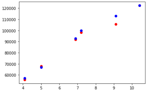
Visualizing Testing Accuracy
In this visualization, the red and blue markers that correspond to actual and predicted data respectively are a bit closer than in the previous example. As a result, this confirms that we achieved higher accuracy using K Cross Validation and GridSearchCV.
In [13]:
fig, ax = plt.subplots()
ax.scatter(X_test,y_test, color = "red")
ax.scatter(X_test,y_pred, color = "blue")
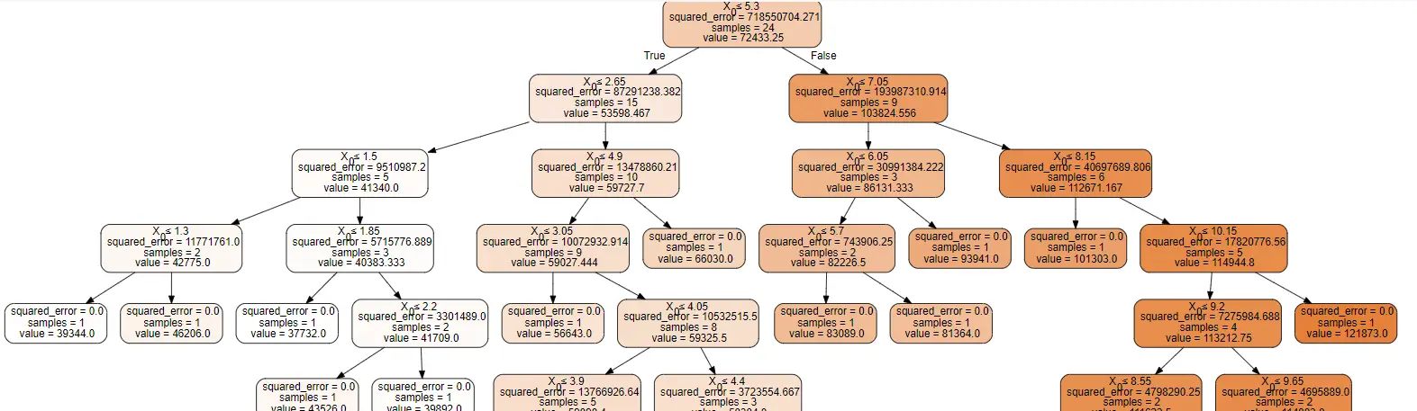
Visualizing Regression Decision Tree with Graphviz
We can visualize the decision tree itself by using the tree module of sklearn and Graphviz package as shown below. (Graphviz can be installed with pip command)
In [14]:
from sklearn import tree
import graphviz

dot_data = tree.export_graphviz(dt_regressor,out_file=None,
                      filled=True, rounded=True,
                      special_characters=True)

graph = graphviz.Source(dot_data)
graph