
Introduction
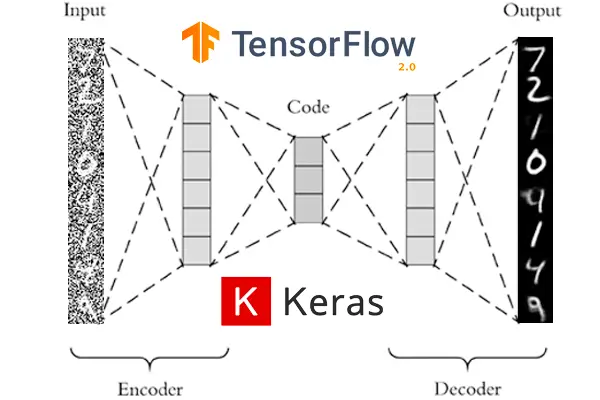
In this tutorial, we will talk about Autoencoders in Keras for beginners. We will give a gentle introduction to autoencoder architecture and cover their applications. Then we will see its differences with GANs (Generative Adversarial Network) and finally show you how to create an autoencoder in Keras.
What are Autoencoders?
Based on the unsupervised neural network concept, Autoencoders is a kind of algorithm that accepts input data, performs compression of the data to convert it to latent-space representation, and finally attempts is to rebuild the input data with high precision.
Autoencoder Architecture
Autoencoder generally comprises of two major components:-
- Encoder – This section takes the input data and then performs the compression of it for obtaining the data in latent-space.
- Decoder – The decoder component follows the encoder in the architecture, it takes the output generated by the encoder and then tries to reconstruct the actual input
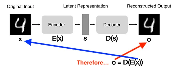
In the above illustration, initially, a digit is provided as an input to the autoencoder. The encoder creates a smaller and compressed version of the input through the latent representation of the digit. Lastly, the operations of the decoder take place, whose aim is to produce copies of input by minimizing the mean squared error between the actual input (available as a dataset) and duplicate input (produced by the decoder).
The experiments have shown that the autoencoder generally produces the input almost identical to the actual input.
Autoencoders vs GANs
- In the case of autoencoders, learning takes place by performing comparisons of input to the output. This method proves beneficial in cases where hidden representations have to be understood but when we try to generate new data, then autoencoders fail.
- On the other hand, GANs have two different networks. The task of determining the difference between real data and generated data is assigned to that network, also called a discriminator. The aim of the generator network is to generate such images that can fool the discriminator and make it believe that the generated images are real images.
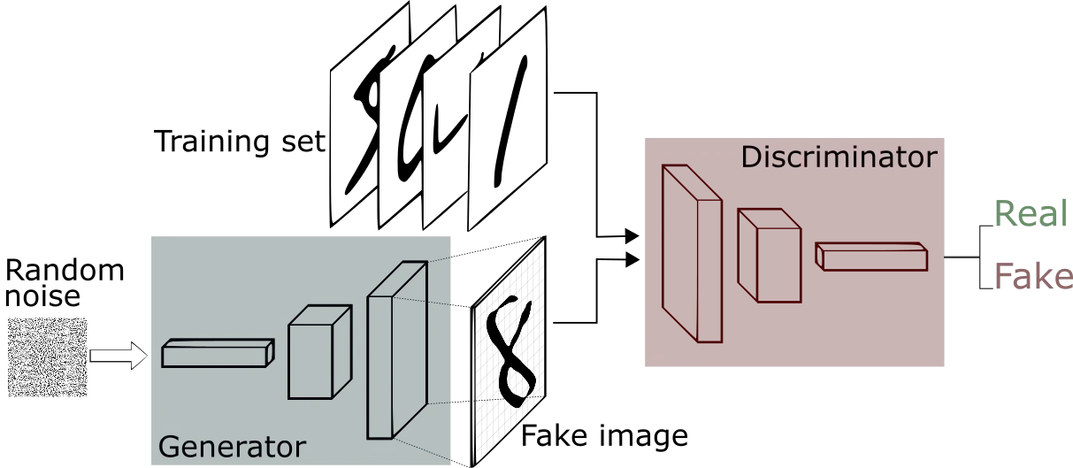
- Autoencoders are not best suited for the image generation method when compared to GANs where for instance, we can generate stunning new images on the basis of the input images provided to the GANs.
Based on the task at our hands, we can either use Autoencoders or GANs. Generally, when we are required to compress data, we can use Autoencoders. When you are required to generate data, you can use GANs.
Applications of Autoencoders
With such innovative functioning, let’s have a look at the applications of Autoencoders and learn how it can be used in various domains.
The applications of Autoencoders are as follows:-
1. Dimensionality Reduction
The traditional method for dimensionality reduction is principal component analysis but autoencoders have been much more powerful and intelligent.
2. Denoising
Denoising is a technique used for removing noise i.e. errors from image data. Along with this, denoising also helps in preprocessing of the images. In case of optical character recognition applications, denoising is majorly done with the help of autoencoders.
3. Anomaly Detection
Anomaly Detection or mislabeled data points identification is an important method for finding out data points that are not complying with other points of the dataset.
4. Image Generation
A variant of Autoencoders i.e. Variational Autoencoder is used for generating new images that are similar to the input images.
5. Sequence to Sequence Prediction
An application of Natural Language Processing that can be achieved by using autoencoders. The sequence to sequence prediction is used for Machine Translation. Apart from this, it can predict the future frames of a video.
6. Recommendation Systems
Autoencoders have great applications in building recommendation systems as well. Recommendation Systems are used for recommending movies, series, songs, products, etc. to different users based on their purchase history, likes, and interests. Here in recommendation systems, users are clustered on the basis of their interests. In case of autoencoders, interests are identified by the encoder and then the decoder tries to predict these interests.
Building an Autoencoders in Keras
Let us now see how to build Autoencoders in Keras. For understanding the complete functionality, we’ll be building each and every component and will use the MNIST dataset as an input.
Here we provide input images, then we perform encoding and decoding by adding dense layers.
Then we build a model for autoencoders in Keras library.
import keras
from keras import layers

# This is the size of our encoded representations
encoding_dim = 32  # 32 floats -> compression of factor 24.5, assuming the input is 784 floats

# This is our input image
input_img = keras.Input(shape=(784,))
# "encoded" is the encoded representation of the input
encoded = layers.Dense(encoding_dim, activation='relu')(input_img)
# "decoded" is the lossy reconstruction of the input
decoded = layers.Dense(784, activation='sigmoid')(encoded)

# This model maps an input to its reconstruction
autoencoder = keras.Model(input_img, decoded)
Here we are creating an encoder model.
# This model maps an input to its encoded representation
encoder = keras.Model(input_img, encoded)
Now we will create the decoder.
# This is our encoded (32-dimensional) input
encoded_input = keras.Input(shape=(encoding_dim,))
# Retrieve the last layer of the autoencoder model
decoder_layer = autoencoder.layers[-1]
# Create the decoder model
decoder = keras.Model(encoded_input, decoder_layer(encoded_input))
With the below code snippet, we’ll be training the autoencoder by using binary cross entropy loss and adam optimizer
autoencoder.compile(optimizer='adam', loss='binary_crossentropy')
Let us now get our input data ready, the MNIST digits dataset is imported and also its labels are removed.
from keras.datasets import mnist
import numpy as np
(x_train, _), (x_test, _) = mnist.load_data()
Also, normalization is performed, this will help in ranging all the values between 0 and 1. We will also flatten the 28×28 images for vectorizing them.
x_train = x_train.astype('float32') / 255.
x_test = x_test.astype('float32') / 255.
x_train = x_train.reshape((len(x_train), np.prod(x_train.shape[1:])))
x_test = x_test.reshape((len(x_test), np.prod(x_test.shape[1:])))
print(x_train.shape)
print(x_test.shape)
Now let is fit our autoencoder model with the epochs of 50.
autoencoder.fit(x_train, x_train,
                epochs=50,
                batch_size=256,
                shuffle=True,
                validation_data=(x_test, x_test))
Verifying Results of our Autoencoder
Once these 50 epochs are completed, we can look at the training or validation loss achieved by the autoencoder model.
The reconstructed inputs and encoded representations can be visualized using Matplotlib.
# Encode and decode some digits
# Note that we take them from the *test* set
encoded_imgs = encoder.predict(x_test)
decoded_imgs = decoder.predict(encoded_imgs)
# Use Matplotlib
import matplotlib.pyplot as plt

n = 10  # How many digits we will display
plt.figure(figsize=(20, 4))
for i in range(n):
    # Display original
    ax = plt.subplot(2, n, i + 1)
    plt.imshow(x_test[i].reshape(28, 28))
    plt.gray()
    ax.get_xaxis().set_visible(False)
    ax.get_yaxis().set_visible(False)

    # Display reconstruction
    ax = plt.subplot(2, n, i + 1 + n)
    plt.imshow(decoded_imgs[i].reshape(28, 28))
    plt.gray()
    ax.get_xaxis().set_visible(False)
    ax.get_yaxis().set_visible(False)
plt.show()
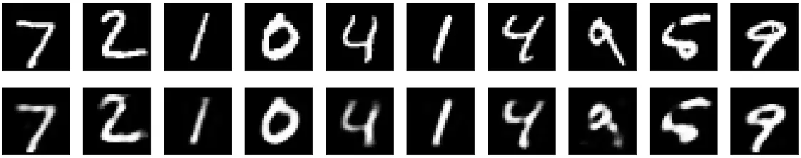
The Output shows that our autoencoder was able to get results (below) similar to the input (top)
- Also Read – Different Types of Keras Layers Explained for Beginners
- Also Read – Keras Dropout Layer Explained for Beginners
- Also Read – Keras Dense Layer Explained for Beginners
- Also Read – Keras Convolution Layer – A Beginner’s Guide
- Also Read – Beginners’s Guide to Keras Models API
- Also Read – Types of Keras Loss Functions Explained for Beginners
Conclusion
It’s time to end the tutorial, where saw how to build Autoencoders in Keras. Besides, we learned about autoencoder architecture along with its several applications. Lastly, we also understood how autoencoders are different compared to GANs.
Reference Keras Documentation

