
Introduction
In this article, we will go through the Seaborn Histogram Plot tutorial that will be helpful to visualize data distribution in your data science and machine learning projects. We will cover many examples in this tutorial for creating different types of histogram plots using the Seaborn histplot() function. We will also tell you the significance of different parameters that are used in the Seaborn Histogram function. So let’s start this tutorial.
Seaborn Histogram Plot Tutorial
The histogram is a way to visualize data distribution with the help of one or more variables. Histogram uses bins for observations count.
Syntax of Histogram Function in Seaborn
The following section shows the syntax and parameters of the Seaborn histogram function i.e. histplot() –
seaborn.histplot(data=None, *, x=None, y=None, hue=None, weights=None, stat=’count’, bins=’auto’, binwidth=None, binrange=None, discrete=None, cumulative=False, common_bins=True, common_norm=True, multiple=’layer’, element=’bars’, fill=True, shrink=1, kde=False, kde_kws=None, line_kws=None, thresh=0, pthresh=None, pmax=None, cbar=False, cbar_ax=None, cbar_kws=None, palette=None, hue_order=None, hue_norm=None, color=None, log_scale=None, legend=True, ax=None, kwargs)**
Parameters Information
- data : pandas.DataFrame, numpy.ndarray, mapping, or sequence – Here we provide the input data for the visualization
- x, y : vectors or keys in data – Through this parameter, we mention the x and y axes positions.
- hue : vector or key in data – This parameter helps in mapping of variables to color for plot.
- weights : vector or key in data – Weights help in understanding the impact of each data point for each bin’s count.
- stat : {“count”, “frequency”, “density”, “probability”} – These are the four types of statistic method that can be used for computing bin values.
- bins : str , number, vector, or a pair of such values – It’s the bin parameter used for specifying the number of bins.
- binwidth : umber or pair of numbers – Here we can set the width of the bin
- binrange : pair of numbers or a pair of pairs – Through this parameter, the lowest and highest value can be specified for edges.
- palette: string, list, dict, or matplotlib.colors.Colormap – We can choose the colors for mapping hue semantic.
- color : matplotlib color – This parameter enables us to choose a single color in case there is no hue mapping.
- kwargs – These are the keyword arguments
The histplot() returns a matplotlib axes with a plot.
Importing the Library
Now we will import the Seaborn library.
import seaborn as sns
Univariate Distribution Histogram in Seaborn
In this type of histogram, we are assigning a variable to ‘x’ for plotting univariate distributions over the x-axis.
We will be using the in-built datasets of seaborn for visualization purposes. So let’s look at different examples of histograms.
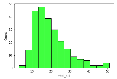
Example 1: Simple Seaborn Histogram Plot (Vertical)
The vertical histogram is the simplest and most common type of histogram you will come across in regular use.
We have loaded the tips dataset using seaborn’s load_dataset function. Now after looking at the initial values with the help of head() function, we will plot a simple histogram.
tips = sns.load_dataset("tips")

tips.head()
Apart from the parameters like data and x, we are using the color parameter to specify the color of the histogram
sns.histplot(data=tips, x="total_bill", color="lime")
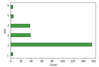
Example 2: Horizontal Histogram
This example shows how we can plot a horizontal histogram using the histplot() function of Seaborn. Note here that we are passing the value to the y parameter to make the histogram plot horizontal
sns.histplot(data=tips, y="size", color = "green")
Different Usages of bin
Bin Width is an important parameter for a histogram to visualize it more effectively for better data analysis. In the following examples, we will play with the binwidth parameter of the seaborn histplot function.
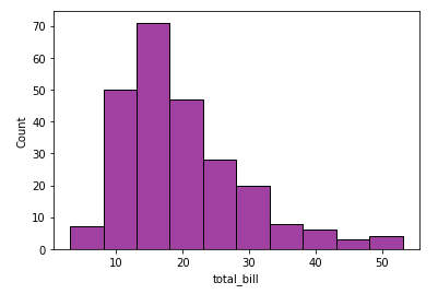
Example 3: Using binwidth parameter of Seaborn histplot()
Here in this example, we will specify the bin width which will enable more control over the distribution of the values in the histogram. In this case, binwidth is passed as 5
sns.histplot(data=tips, x="total_bill", binwidth=5, color="purple")
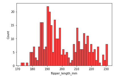
Example 4: Using bins values in Seaborn histplot()
The second example in this category is the one where we are mentioning the number of bins to be used for placing all the data in it.
Here the data used will be about penguins. Let’s load the data and then use it for the purpose of visualization.
penguins = sns.load_dataset("penguins")

penguins.head()
sns.histplot(data=penguins, x="flipper_length_mm", bins=50,color="red")
Categorizing the bins
The third kind of histogram will showcase how we can categorize the bins based on different sets of variables present. For this purpose, we’ll use the hue parameter of histplot() function.
For this example another dataset is used, it’s titled ‘mpg’.
mpg = sns.load_dataset("mpg")

mpg.head()
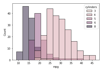
Example 5: Layered Categorization of Histogram Bins using Hue in Seaborn
Here the seaborn histogram is structured in form of layers. As you can see the categorization is done using “cylinders” attribute of the dataset which is passed to hue parameter.
sns.histplot(data=mpg, x="mpg", hue="cylinders")
Output
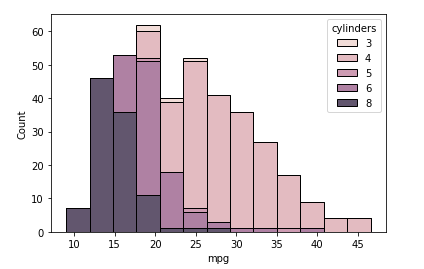
Example 6: Categorization of Histogram Bins using Hue and Stack
In this example, we are stacking the categories for better visualization. So let’s see how it is displayed. For implementing the stack feature, we can use the multiple parameter of histplot function.
sns.histplot(data=mpg, x="mpg", hue="cylinders", multiple="stack")
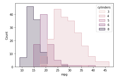
Example 7: Categorization of Histogram Bins using Hue and Step
In this example, we will create the histogram in step form. For this, we have to use the element parameter of the seaborn histplot function where we pass the argument “step”
sns.histplot(mpg, x="mpg", hue="cylinders", element="step")
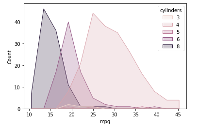
Example 8: Polygon Shaped Histogram in Seaborn
This kind of histogram is the one where we can shape the histogram as polygons using the element parameter passing poly as the value.
sns.histplot(mpg, x="mpg", hue="cylinders", element="poly")
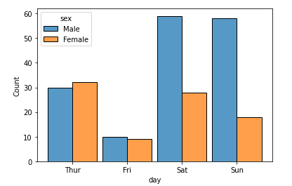
Example 9: Seaborn Histogram for Comparison
The previous examples of histograms showed how we can visualize the distribution of continuous or discrete values. In this example, we’ll look at how categorical values can be visualized in the histogram.
For this example, we use multiple parameter in which dodge value is passed. The shrink parameter is used for either increasing or decreasing the size of histogram bars. The range for this parameter lies between 0 to 1.
Remember lower values result in thin histograms but higher values will produce thicker histogram bars.
sns.histplot(data=tips, x="day", hue="sex", multiple="dodge", shrink=.9)
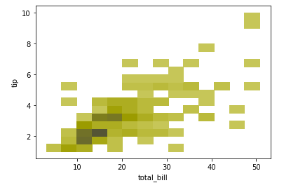
Bivariate Histogram
This is the second type of histogram that we can build. Here the bivariate histogram uses two different variables and then plots them with the help of the x and y-axis.
Example 10: Simple Bivariate Histogram in Seaborn
sns.histplot(tips, x="total_bill", y="tip", color = "yellow")
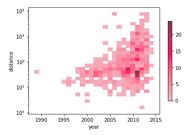
Example 11: Bivariate Histogram with Colorbar
This example shows a bivariate histogram with bin values that also contains a color bar to represent the values. For displaying color bar, we will add colormap for the same.
In the below code, we are using planets dataset. We then specify the x and y variables along with the bins, discrete, log_scale parameters. We also specify the cbar parameter to attach the color bar to the plot.
The discrete variable is used for handling the gaps that may arise in the histogram and log_scale parameter is used for setting a log_scale on data axis.
planets = sns.load_dataset("planets")
sns.histplot(
    planets, x="year", y="distance",
    bins=30, discrete=(True, False), log_scale=(False, True),
    cbar=True, cbar_kws=dict(shrink=.75),color="pink"
)
Conclusion
In this article, we went through the Seaborn Histogram Plot tutorial using histplot() function. We saw various types of examples of creating histograms for univariate and multivariate scenarios and also with various types of binning techniques.
Reference: https://seaborn.pydata.org/

