Introduction
Cost functions in machine learning are functions that help to determine the offset of predictions made by a machine learning model with respect to actual results during the training phase. These are used in those supervised learning algorithms that use optimization techniques. Notable examples of such algorithms are regression, logistic regression, neural network, etc. You can understand more about optimization at the below link.
- Also Read – Understanding Optimization in Machine Learning with Animation
- Also Read – Types of Keras Loss Functions Explained for Beginners
Cost functions are also known as Loss functions. There are many cost functions in machine learning and each has its own use cases depending on whether it is a regression problem or classification problem. But let us first have a closer look at cost function.
Why Cost Functions in Machine Learning
During the training phase, the model assumes the initial weights randomly and tries to make a prediction on training data. But how will the model get to know how much “far” it was from the prediction? It definitely needs this information so that it can adjust the weight accordingly (using gradient descent) in the next iteration on training data.
This is where cost function comes into the picture. Cost function is a function that takes both predicted outputs by the model and actual outputs and calculates how much wrong the model was in its prediction.
Now with this quantifiable information from cost function, the model tries to adjust it’s weight for the next iteration on training data so that the error given by cost function gets further reduced. The goal of the training phase is to come up with weights that minimize this error in each iteration to the point where it can’t be reduced further. This is essentially an optimization problem.
Now let us see what are the different types of cost functions in machine learning.
Cost functions for Regression problems
In regression, the model predicts an output value for each training data during the training phase. The cost functions for regression are calculated on distance-based error. Let us first understand this concept first.
Initial Concept – Distance Based Error
Let us say that for a given set of input data, the actual output was y and our regression model predicts y’ then the error in prediction is calculated simply as
Error = y-y’
This also known as distance-based error and it forms the basis of cost functions that are used in regression models. Below animation gives a more clear geometrical interpretation of distance-based error.
Having built the concept of distance-based error let us see the various cost functions for regression models.
Mean Error (ME)
In this cost function, the error for each training data is calculated and then the mean value of all these errors is derived. Calculating mean of the errors is the simplest and most intuitive way possible. But there is a catch here.
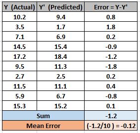
The errors can be both negative or positive and during summation, they will tend to cancel each other out. In fact, it is theoretically possible that the errors are such that positive and negatives cancel each other to give zero error mean error for the model.
So Mean Error is not a recommended cost function for regression. But it does lay the foundation for our next cost functions.
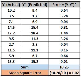
Mean Squared Error (MSE)
This improves the drawback we saw in Mean Error above. Here a square of the difference between the actual and predicted value is calculated to avoid any possibility of negative error.
So in this cost function, MSE is calculated as mean of squared errors for N training data.
MSE = (Sum of Squared Errors)/N
The below example should help you to understand MSE much better. MSE is also known as L2 loss.
Mean Absolute Error (MAE)
This also addresses the shortcoming of ME in a different way. Here an absolute difference between the actual and predicted value is calculated to avoid any possibility of negative error.
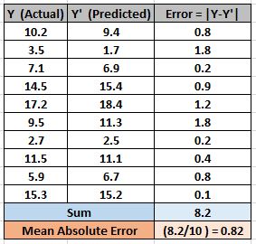
So in this cost function, MAE is calculated as the mean of absolute errors for N training data.
MAE = (Sum of Absolute Errors)/N
The below example shows how MAE is calculated. MAE is also known as L1 Loss.
MSE Vs MAE – Which one to choose?
Both MSE and MAE avoids the problem of negative errors canceling each other in case of ME. So does it mean we can use any one of them at our will? Well not really !! To understand this we have to first understand the nature of MSE.
MSE penalizes small errors
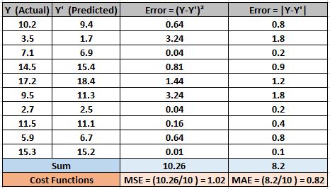
In MSE, since each error is squared, it helps to penalize even small deviations in prediction when compared to MAE.
The below comparison should give you a better understanding of this comparison. As you can see, for example, the absolute error of 1.8 is penalized to higher error 3.24 when squared. And this penalized effect is also seen on overall MSE, compared to MAE.
MSE has an adverse effect on Outliers
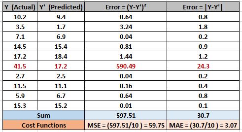
So now you might be thinking that MSE has supremacy over MAE. But wait.. there is a flip side as well with penalizing of errors. What if, your data has outliers that contribute to larger prediction errors. Now if you square this error further, it will magnify much more and also increase the final MSE error.
In the below example, we have introduced an outlier in the data(marked in red ) and you can see that there is such a huge difference between its absolute error and squared error. The squared error is so huge that it also increases the overall MSE. This MSE error is very big compared to MAE.
So coming back to our original question which should be used – MSE or MAE. Well, it depends on your data –
- If your data has noise or outliers, then overall MSE will be amplified which is not good. In this case, it is better to use MAE.
- If your data is free from noise or outliers, then it is good to use MSE as it will rightly penalize the errors in prediction much better than MAE.
[adrotate banner=”3″]
Cost functions for Classification problems
Cost functions used in classification problems are different than what we saw in the regression problem above. There is a reason why we don’t use regression cost functions for classification problem and we will see it later. But before that let us see the classification cost functions.
Initial Concept – Cross Entropy Intuition
The name cross entropy might give you a bummer at first, but let me give you a very intuitive understanding. Cross Entropy can be considered as a way to measure the distance between two probability distributions. (This is an intuitive understanding, however, as it does not really measure the distance between the probability distribution in mathematics term)
So how does cross entropy help in the cost function for classification? Let us understand this with a small example.
Let us consider that we have a classification problem of 3 classes as follows.
Class(Orange,Apple,Tomato)
The machine learning model will actually give a probability distribution of these 3 classes as output for a given input data. The class having the highest probability is considered as a winner class for prediction.
Output = [P(Orange),P(Apple),P(Tomato)]
The actual probability distribution for each class is shown below.
Orange = [1,0,0]
Apple = [0,1,0]
Tomato = [0,0,1]
During the training phase, for example, if the training data is Orange, the predicted probability distribution should tend towards the actual probability distribution of Orange. If predicted probability distribution is not closer to the actual one, the model has to adjust its weight.
This is where cross entropy becomes a tool to calculate how much far is the predicted probability distribution from the actual one. This intuition of cross entropy is shown in the below animation.
This was just an intuition behind cross entropy. It has it’s origin from information theory and you can read here to get more insight on this topic.
Now with this understanding of cross entropy, let us now see the classification cost functions.
Categorical Cross Entropy Cost Function
This cost function is used in the classification problems where there are multiple classes and input data belongs to only one class.
Before defining the cost function let us first understand how cross entropy is calculated.
Let us assume the model gives the probability distribution as below for M classes for a particular input data D.
P(D) = [y1′ , y2′ , y3′ … yM’]
And the actual or target probability distribution of the data D is
A(D) = [y1 , y2 , y3 … yM]
Then cross entropy for that particular data D is calculated as
CrossEntropy(A,P) = – ( y1*log(y1′) + y2*log(y2′) + y3*log(y3′) + … + yM*log(yM’) )
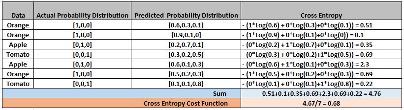
Let us quickly understand this with the help of above example where .
P(Orange) = [0.6, 0.3, 0.1]
A(Orange) = [1, 0, 0]
Cross_Entropy(A,P) = – (1*Log(0.6) + 0*Log(0.3)+0*Log(0.1)) = 0.51
The above formula just measures the cross entropy for a single observation or input data.
The error in classification for the complete model is given by categorical cross entropy which is nothing but the mean of cross entropy for all N training data.
Categorical_Cross_Entropy = (Sum of Cross Entropy for N data)/N
The below example will help you understand Categorical Cross Entropy better.
Binary Cross Entropy Cost Function
Binary cross entropy is a special case of categorical cross entropy when there is only one output which just assumes a binary value of 0 or 1 to denote negative and positive class respectively
Let us assume that actual output is denoted by a single variable y, then cross entropy for a particular data D is can be simplified as follows –
cross_entropy(D) = – y*log(y’) when y = 1
cross_entropy(D) = – (1-y)*log(1-y’) when y = 0
The error in binary classification for the complete model is given by binary cross entropy which is nothing but the mean of cross entropy for all N training data.
Binary_Cross_Entropy = (Sum of Cross_Entropy for N data)/N
Why Cross Entropy and Not MAE/MSE in Classification?
We could have used regression cost function MAE/MSE even for classification problems. But yet we decided to go with seemingly complicated cross entropy. And there has to be a reason behind this. Let us see why.
Overconfident wrong prediction
Sometimes machine learning model, especially during the training phase not only makes a wrong classification but makes it with so confidence that they deserve much more penalization.
Just to give you a feel of this, imagine a model classifying a male’s medical condition as pregnancy with 0.9 probability whereas actual probability is 0. So it is not only doing wrong classification but doing it with ridiculous overconfidence.

Penalization of overconfident wrong prediction
Such models deserve severe penalization during the training phase. For simplicity purpose let us see how binary Cross Entropy, MAE and MSE penalize in such a situation.
In the below example, the two scenarios of y=1, y’=0.2 and y=0, y’=0.8 are an example of confidently wrong classification. As we can see Binary Cross Entropy is doing a more severe penalty than MAE or MSE for this situation.
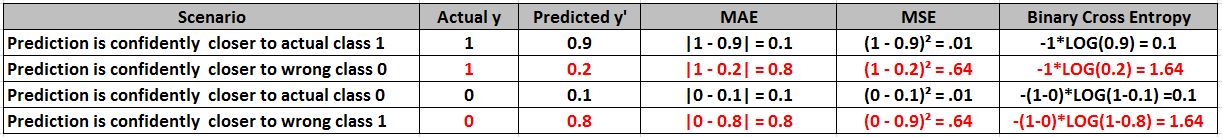
Binary cross entropy penalizes confidently wrong prediction more severely because of its intrinsic characteristics.
The below illustration shows the graph for binary cross entropy function for the two scenarios of actual y=1 and y=0. In both cases, you can see cost reaching towards infinity as predicted probability becomes more and more wrong.
So the capability of cross entropy to punish confident wrong predictions makes it a good choice for classification problems.
Hinge Loss Function
Hinge loss is another cost function that is mostly used in Support Vector Machines (SVM) for classification. Let us see how it works in case of binary SVM classification
To work with hinge loss, the binary classification output should be denoted with +1 or -1.
SVM predicts a classification score h(y) where y is the actual output. Then hinge loss for a particular data D is given as-
Hinge_Loss(D) = max(0,1-y*h(y))
Then hinge loss cost function for the entire N data set is given by
Hinge_Loss_Cost = Sum of Hinge loss for N data points
The below example will give you more clarity about Hinge Loss.
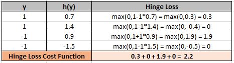
Similarly to cross entropy cost function, hinge loss penalizes those predictions which are wrong and overconfident.
As you can see in the below illustration, as soon as prediction starts deviating much from the expected output of +1 or -1, the incurred cost also starts ascending.
A quick summary
- Cost functions in machine learning, also known as loss functions, calculates the deviation of predicted output from actual output during the training phase.
- Cost functions are an important part of the optimization algorithm used in the training phase of models like logistic regression, neural network, support vector machine.
- There are many cost functions to choose from and the choice depends on type of data and type of problem (regression or classification).
- Mean squared error (MSE) and Mean Absolute Error (MAE) are popular cost functions used in regression problems.
- For classification problems, the models which give probability output mostly use categorical cross entropy and binary cross entropy cost functions.
- SVM, another classification model uses Hinge Loss as its cost function
- Also Read – Types of Keras Loss Functions Explained for Beginners
- Also Read- Demystifying Confusion Matrix and Performance Metrics in Machine Learning
- Also Read- Overfitting and Underfitting in Machine Learning – Animated Guide for Beginners
In the End…
So this was our humble attempt to make you aware about the world of different cost functions in machine learning, in the most simplest and illustrative way as possible. I really hope you found this post very helpful.
Do share your feedback about this post in the comments section below. If you found this post informative, then please do share this and subscribe to us by clicking on the bell icon for quick notifications of new upcoming posts. And yes, don’t forget to join our new community MLK Hub and Make AI Simple together.