
Introduction
In this tutorial, we will show the implementation of PCA in Python Sklearn (a.k.a Scikit Learn ). First, we will walk through the fundamental concept of dimensionality reduction and how it can help you in your machine learning projects. Next, we will briefly understand the PCA algorithm for dimensionality reduction. Finally, we will explain to you an end-to-end implementation of PCA in Sklearn with a real-world dataset.
1. Curse of Dimensionality in Machine Learning
The curse of dimensionality in machine learning refers to the issues that arise due to high dimensionality in the dataset. In layman’s terms, dimensionality may refer to the number of attributes or fields in the structured dataset. In the case of an image the dimension can be considered to be the number of pixels, and so on.
Often in real-world machine learning problems, the dataset may contain hundreds of dimensions and in some cases thousands. Although more dimension means more data to work with, it leads to the following curse of dimensionality –
- Humans cannot visualize data beyond 3-Dimension. Hence it is very challenging to visualize and analyze data having a very high dimensionality.
- It may take a lot of computational resources to process a high dimension data with machine learning algorithms.
- The ML model generated with high dimension data set may not show good accuracy or suffer from overfitting.
2. What is Dimensionality Reduction?
Dimensionality reduction refers to the various techniques that can transform data from high dimension space to low dimension space without losing the information present in the data. It is essentially a way to avoid the curse of dimensionality that we discussed above.
Advantages of Dimensionality Reduction
You may like to apply dimensionality reduction on the dataset for the following advantages-
- It reduces the computational time required for training the ML model.
- It becomes easier to visualize data in 2D or 3D plot for analysis purpose
- It eliminates redundancy present in data and retains only relevant information
Dimensionality Reduction Techniques
The various methods used for dimensionality reduction include:
- Principal Component Analysis (PCA)
- Linear Discriminant Analysis (LDA)
- Generalized Discriminant Analysis (GDA)
In this article, we will be only looking only at the PCA algorithm and its implementation in Sklearn
3. What is PCA?
The Principal Component Analysis (PCA) is a multivariate statistical technique, which was introduced by an English mathematician and biostatistician named Karl Pearson.
In this method, we transform the data from high dimension space to low dimension space with minimal loss of information and also removing the redundancy in the dataset.
While applying PCA, the high dimension data is mapped into a number of components which is the input hyperparameter that should be provided. The number of components has to be less than equal to the dimension of the data. These components hold the information of the actual data in a different representation such that 1st component holds the maximum information followed by 2nd component and so on.
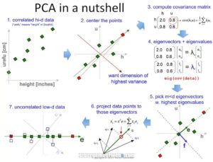
Steps involved in PCA
At a high level, the steps involved in PCA are –
- Standardization of the dataset is a must before applying PCA because PCA is quite sensitive to the dataset that has a high variance in its values.
- Compute the covariance matrix
- Calculate Eigenvalues and Eigenvectors using the covariance matrix of the previous step to identify principal components.
- Sort the Eigenvalues and its Eigenvectors in descending order. Here the eigenvector with the highest value has the highest significance and forms the first principal component, and so on. So if we choose to take components n = 2, the top two eigenvectors will be selected.
- Transform the original matrix of data by multiplying it top n eigenvectors selected above.
The Scikit Learn implementation of PCA abstracts all this mathematical calculation and transforms the data with PCA, all we have to provide is the number of principal components we wish to have.
4. Overview of our PCA Example
In this example of PCA using Sklearn library, we will use a highly dimensional dataset of Parkinson disease and show you –
- How PCA can be used to visualize the high dimensional dataset.
- How PCA can avoid overfitting in a classifier due to high dimensional dataset.
- How PCA can improve the speed of the training process.
So let us begin.
About Dataset
We are using a Parkinson’s disease dataset that contains 754 attributes and 756 records. As you can see it is highly dimensional with 754 attributes. It contains an attribute ‘class’ that contains 0 and 1 to denote the absence or presence of Parkinson’s disease.
The dataset can be downloaded from here.
Importing necessary libraries
We first load the libraries required for this example.
In[0]:
from sklearn.decomposition import PCA
from sklearn.preprocessing import StandardScaler
from sklearn.model_selection import train_test_split
import pandas as pd
from sklearn.linear_model import LogisticRegression
from sklearn.metrics import accuracy_score
import matplotlib.pyplot as plt
import warnings
warnings.filterwarnings('ignore')
Reading the CSV Dataset
Next, we read the dataset CSV file using Pandas and load it into a dataframe. We will do a quick check if the dataset got loaded properly by fetching the 5 records using the head function. We also validate the number of rows and columns by using shape property of the dataframe.
Finally, we calculate the count of the two classes 0 and 1 in the dataset.
In [1]:
df= pd.read_csv(r"pd_speech_features.csv")

df.head()
Out[1]:
| gender | PPE | DFA | RPDE | numPulses | numPeriodsPulses | meanPeriodPulses | stdDevPeriodPulses | locPctJitter | locAbsJitter | … | tqwt_kurtosisValue_dec_28 | tqwt_kurtosisValue_dec_29 | tqwt_kurtosisValue_dec_30 | tqwt_kurtosisValue_dec_31 | tqwt_kurtosisValue_dec_32 | tqwt_kurtosisValue_dec_33 | tqwt_kurtosisValue_dec_34 | tqwt_kurtosisValue_dec_35 | tqwt_kurtosisValue_dec_36 | class | |
|---|---|---|---|---|---|---|---|---|---|---|---|---|---|---|---|---|---|---|---|---|---|
| 0 | 1 | 0.85247 | 0.71826 | 0.57227 | 240 | 239 | 0.008064 | 0.000087 | 0.00218 | 0.000018 | … | 1.5620 | 2.6445 | 3.8686 | 4.2105 | 5.1221 | 4.4625 | 2.6202 | 3.0004 | 18.9405 | 1 |
| 1 | 1 | 0.76686 | 0.69481 | 0.53966 | 234 | 233 | 0.008258 | 0.000073 | 0.00195 | 0.000016 | … | 1.5589 | 3.6107 | 23.5155 | 14.1962 | 11.0261 | 9.5082 | 6.5245 | 6.3431 | 45.1780 | 1 |
| 2 | 1 | 0.85083 | 0.67604 | 0.58982 | 232 | 231 | 0.008340 | 0.000060 | 0.00176 | 0.000015 | … | 1.5643 | 2.3308 | 9.4959 | 10.7458 | 11.0177 | 4.8066 | 2.9199 | 3.1495 | 4.7666 | 1 |
| 3 | 0 | 0.41121 | 0.79672 | 0.59257 | 178 | 177 | 0.010858 | 0.000183 | 0.00419 | 0.000046 | … | 3.7805 | 3.5664 | 5.2558 | 14.0403 | 4.2235 | 4.6857 | 4.8460 | 6.2650 | 4.0603 | 1 |
| 4 | 0 | 0.32790 | 0.79782 | 0.53028 | 236 | 235 | 0.008162 | 0.002669 | 0.00535 | 0.000044 | … | 6.1727 | 5.8416 | 6.0805 | 5.7621 | 7.7817 | 11.6891 | 8.2103 | 5.0559 | 6.1164 | 1 |
5 rows × 754 columns
In [2]:
df.shape
Out[2]:
(756, 754)
In [3]:
df['class'].value_counts()
Out[3]:
1    564
0    192
Name: class, dtype: int64
5. Visualizing High Dimensional Dataset with PCA using Sklearn
As we discussed earlier, it is not possible for humans to visualize data that has more than 3 dimensional. In this dataset, there are 754 dimensions. Let us reduce the high dimensionality of the dataset using PCA to visualize it in both 2-D and 3-D.
Standardizing the Dataset
It is compulsory to standardize the dataset before applying PCA, otherwise, it will produce wrong results.
Here we are using StandardScaler() function of sklearn.preprocessing module to standardize both train and test datasets.
In [4]:
X_Scale = scaler.transform(X)
- Also Read – Why to do Feature Scaling in Machine Learning
Applying PCA with Principal Components = 2
Now let us apply PCA to the entire dataset and reduce it into two components. We are using the PCA function of sklearn.decomposition module.
After applying PCA we concatenate the results back with the class column for better understanding.
In [5]:
pca2 = PCA(n_components=2)
principalComponents = pca2.fit_transform(X_Scale)

principalDf = pd.DataFrame(data = principalComponents, columns = ['principal component 1', 'principal component 2'])

finalDf = pd.concat([principalDf, df[['class']]], axis = 1)
finalDf.head()
Out[5]:
| principal component 1 | principal component 2 | class | |
|---|---|---|---|
| 0 | -10.184156 | 1.252252 | 1 |
| 1 | -10.621219 | 1.659891 | 1 |
| 2 | -13.507782 | -1.231873 | 1 |
| 3 | -9.277452 | 8.087223 | 1 |
| 4 | -7.142122 | 3.815401 | 1 |
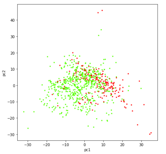
Visualizing Data in 2 Dimension Scatter Plot
Let us now visualize the dataset that has been reduced to two components with the help of a scatter plot.
In [6]:
plt.figure(figsize=(7,7))
plt.scatter(finalDf['principal component 1'],finalDf['principal component 2'],c=finalDf['class'],cmap='prism', s =5)
plt.xlabel('pc1')
plt.y;label('pc2')
Out[6]:
Applying PCA with Principal Components = 3
Just like earlier, let us again apply PCA to the entire dataset to produce 3 components.
In [7]:
pca3 = PCA(n_components=3)
principalComponents = pca3.fit_transform(X_Scale)

principalDf = pd.DataFrame(data = principalComponents, columns = ['principal component 1', 'principal component 2', 'principal component 3'])

finalDf = pd.concat([principalDf, df[['class']]], axis = 1)
finalDf.head()
Out[7]:
| principal component 1 | principal component 2 | principal component 3 | class | |
|---|---|---|---|---|
| 0 | -10.184156 | 1.252253 | -7.185881 | 1 |
| 1 | -10.621219 | 1.659890 | -6.873706 | 1 |
| 2 | -13.507782 | -1.231873 | -7.076563 | 1 |
| 3 | -9.277453 | 8.087221 | 14.467958 | 1 |
| 4 | -7.142122 | 3.815398 | 15.474813 | 1 |
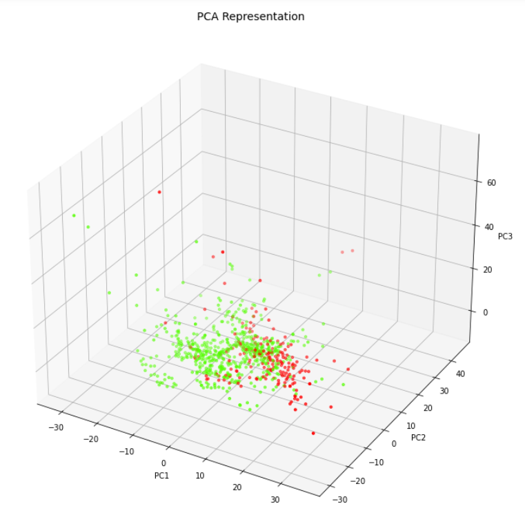
Visualizing Data in 3 Dimension Scatter Plot
Let us visualize the three PCA components with the help of 3-D Scatter plot.
In [8]:
from mpl_toolkits.mplot3d import Axes3D

fig = plt.figure(figsize=(9,9))
axes = Axes3D(fig)
axes.set_title('PCA Representation', size=14)
axes.set_xlabel('PC1')
axes.set_ylabel('PC2')
axes.set_zlabel('PC3')

axes.scatter(finalDf['principal component 1'],finalDf['principal component 2'],finalDf['principal component 3'],c=finalDf['class'], cmap = 'prism', s=10)
Out[8]:
6. Improve Speed and Avoid Overfitting of ML Models with PCA using Sklearn
Now we will see the curse of dimensionality in action. We will create two logistic regression models – first without applying the PCA and then by applying PCA. We will capture their training times and accuracies and compare them.
Splitting dataset into Train and Test Sets
Here we are going to separate the dependent label column into y dataframe. And all remaining columns into X dataframe.
Then we split them into train and test sets in ration of 70%-30% using train_test_split function of Sklearn.
In [9]:
X = df.drop('class',axis=1).values
y = df['class'].values

X_train, X_test, y_train, y_test = train_test_split(X,y, test_size=0.3,random_state=0)
Standardizing the Dataset
This time we apply standardization to both train and test datasets but separately.
In [10]:
scaler = StandardScaler()

# Fit on training set only.
scaler.fit(X_train)

# Apply transform to both the training set and the test set.
X_train_pca = scaler.transform(X_train)
X_test_pca = scaler.transform(X_test)
Creating Logistic Regression Model without PCA
Here we create a logistic regression model and can see that the model has terribly overfitted. The training accuracy is 100% and the testing accuracy is 84.5%.
Also do keep a note that the training time was 151.7 ms here.
In [11]:
%%time

logisticRegr = LogisticRegression()
logisticRegr.fit(X_train,y_train)

y_train_hat =logisticRegr.predict(X_train)
train_accuracy = accuracy_score(y_train, y_train_hat)*100
print('"Accuracy for our Training dataset with PCA is: %.4f %%' % train_accuracy)
Out[11]:
"Accuracy for our Training dataset with PCA is: 100.0000 %
Wall time: 151.7 ms
In [12]:
y_test_hat=logisticRegr.predict(X_test)
test_accuracy=accuracy_score(y_test,y_test_hat)*100
test_accuracy
print("Accuracy for our Testing dataset with tuning is : {:.3f}%".format(test_accuracy) )
Out[12]:
Accuracy for our Testing dataset with tuning is : 84.581%
Creating Logistic Regression Model with PCA
Below we have created the logistic regression model after applying PCA to the dataset. It can be seen that this time there is no overfitting with the PCA dataset. Both training and the testing accuracy is 79% which is quite a good generalization.
Also, here we see that the training time is just 7.96 ms, which is a significant drop from 151.7 ms. It is almost 20 times fast here. You may not appreciate this improvement much because both are in milliseconds but when we are dealing with a huge amount of data, the training speed improvement of this scale becomes quite significant.
In [13]:
%%time

logisticRegr = LogisticRegression()
logisticRegr.fit(X_train_pca,y_train)

y_train_hat =logisticRegr.predict(X_train_pca)
train_accuracy = accuracy_score(y_train, y_train_hat)*100
print('"Accuracy for our Training dataset with PCA is: %.4f %%' % train_accuracy)
Out[13]:
"Accuracy for our Training dataset with PCA is: 79.7732 %
Wall time: 7.96 ms
In [14]:
y_test_hat=logisticRegr.predict(X_test_pca)
test_accuracy=accuracy_score(y_test,y_test_hat)*100
test_accuracy
print("Accuracy for our Testing dataset with PCA is : {:.3f}%".format(test_accuracy) )
Out[15]:
Accuracy for our Testing dataset with PCA is : 79.295%
Conclusion
We hope you liked our tutorial and now better understand how to implement the PCA algorithm using Sklearn (Scikit Learn) in Python. Here, we used an example to show practically how PCA can help to visualize a high dimension dataset, reduces computation time, and avoid overfitting.

