
Introduction
In this article, we will go through the tutorial for TensorBoard which is a visualization tool to understand various metrics of your neural network model and the training process. We will first explain what is TensorBoard and how to install it. Then, we will show you an example of how to use Tensorboard using Keras and go through various visualizations.
What is TensorBoard?
TensorBoard is a visualization web app to get a better understanding of various parameters of the neural network model and its training metrics. Such visualizations are quite useful when you are doing experiments with neural network models and want to keep a close watch on the related metrics. It is open-source and is a part of the Tensorflow group.
Some of the useful things you can do with TensorBoard includes –
- Visualize metrics like accuracy and loss.
- Visualize model graph.
- Visualize histograms for weights and biases to understand how they change during training.
- Visualize data like text, image, and audio.
- Visualize embeddings in lower dimension space.
TensorBoard Tutorial (Keras)
Here we are going to use a small project to create a neural network in Keras for Tensorboard Tutorial. For this, we are going to use the famous MNIST handwritten digit recognition dataset.
Since this is a TensorBoard tutorial, we will not explain much about the data preprocessing and neural network building process. To understand more details about working with MNIST handwritten digit dataset you can check below tutorial –
i) Install TensorBoard
You can install TensorBoard by using pip as shown below –
pip install tensorboard
ii) Starting TensorBoard
The first thing we need to do is start the TensorBoard service. To do this you need to run below in the command prompt. –logdir parameter signifies the directory where data will be saved to visualize TensorBoard. Here we have given the directory name as ‘logs’.
tensorboard --logdir logs
This will start the TensorBoard service at the default port 6066 as shown below. The TesnorBoard dashboard can be accessed as http://localhost:6006/
Output:
Serving TensorBoard on localhost; to expose to the network, use a proxy or pass --bind_all
TensorBoard 2.5.0 at http://localhost:6006/ (Press CTRL+C to quit)
In Jupyer notebook, you can issue the following command in the cell
%tensorboard --logdir logs
iii) Loading Libraries
We will quickly import the required libraries for our example. (Do note these libraries have nothing to do with TensorBoard but are needed for building the neural network of our example.)
import tensorflow as tf
from tensorflow import keras
import matplotlib.pyplot as plt
%matplotlib inline
import numpy as np
iv) Loading MNIST Dataset
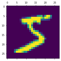
Now we will load the MNIST dataset that comes as part of the Keras package. Let us also quickly visualize one sample data after loading the dataset.
(X_train, y_train) , (X_test, y_test) = keras.datasets.mnist.load_data()
plt.matshow(X_train[0])
Output:
v) Preprocessing
We will now preprocess the data by normalizing it between 0 to 1 and then flattening it.
X_train = X_train / 255
X_test = X_test / 255

X_train_flattened = X_train.reshape(len(X_train), 28*28)
X_test_flattened = X_test.reshape(len(X_test), 28*28)
model = keras.Sequential([
    keras.layers.Flatten(input_shape=(28, 28)),
    keras.layers.Dense(100, activation='relu'),
    keras.layers.Dense(10, activation='sigmoid')
])

model.compile(optimizer='adam',
              loss='sparse_categorical_crossentropy',
              metrics=['accuracy'])
vii) Creating Callback Object
This is where we need to draw our attention while working with TensorBoard. We have to create a Keras callback object for TensorBoard which will help to write logs for TensorBoard during the training process.
Please do note that the parent path for log_dir below should be the same as the logdir value we gave while starting the TensorBoard service in the second step.
tb_callback = tf.keras.callbacks.TensorBoard(log_dir="logs/", histogram_freq=1)
viii) Training Model
Finally, we start the training of the model by using fit() function. We train it for 5 epochs and do notice that we have also passed the callback object that we created in the previous step.
model.fit(X_train, y_train, epochs=5,callbacks=[tb_callback])
Epoch 1/5
1875/1875 [==============================] - 3s 2ms/step - loss: 0.2773 - accuracy: 0.9206
Epoch 2/5
1875/1875 [==============================] - 3s 2ms/step - loss: 0.1255 - accuracy: 0.9627
Epoch 3/5
1875/1875 [==============================] - 3s 2ms/step - loss: 0.0881 - accuracy: 0.9738
Epoch 4/5
1875/1875 [==============================] - 3s 2ms/step - loss: 0.0668 - accuracy: 0.9793
Epoch 5/5
1875/1875 [==============================] - 3s 2ms/step - loss: 0.0528 - accuracy: 0.9840
ix) Visualization Model in Tensorboard
We can now go to the TensorBoard dashboard that we started in the first step and see what all visualizations it has to offer. The visualizations mostly depend on what data you have logged for TensorBoard. Depending on the logged data corresponding TensorBoard plugins get activated and you can see them by selecting ‘Inactive’ dropdown in the top right corner of the dashboard.
Let us see the visualizations available in our example.
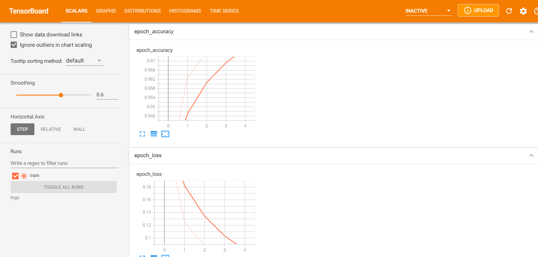
Scalars
It shows visualizations for accuracy and loss in each epoch during the training process. And when you hover the graph it shows more information like value, step, time.
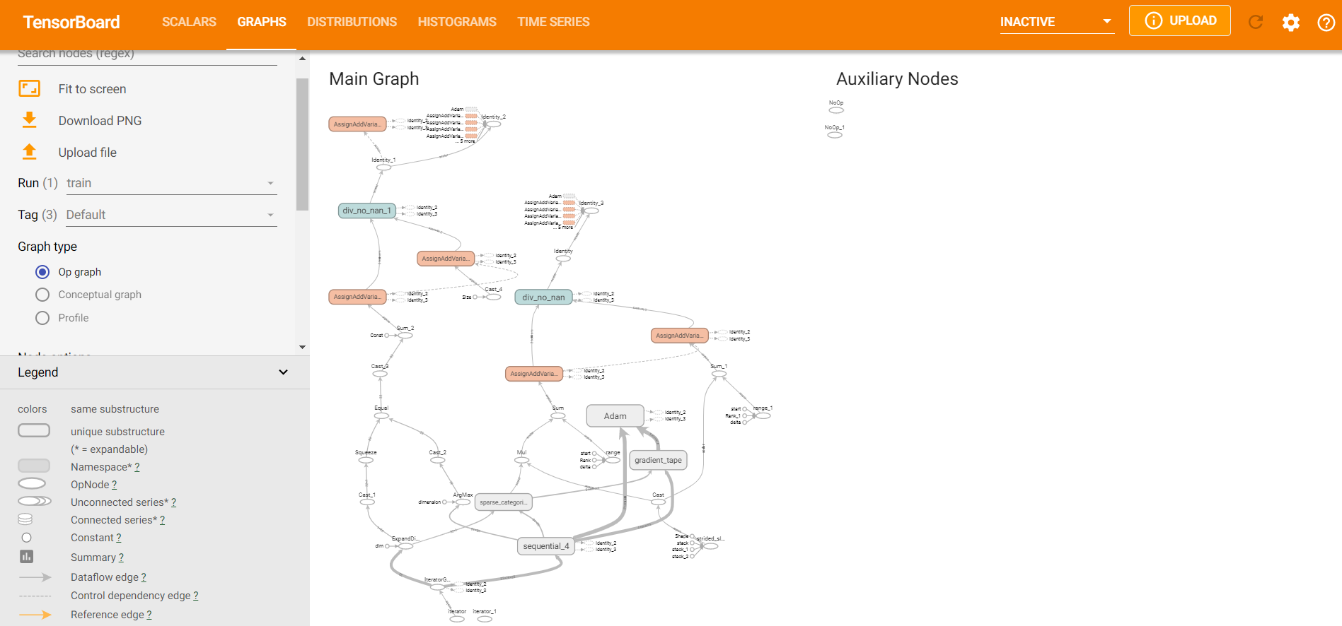
Graph
The neural network model is essentially computational graphs in TensorFlow Keras and it can be visualized in this section.
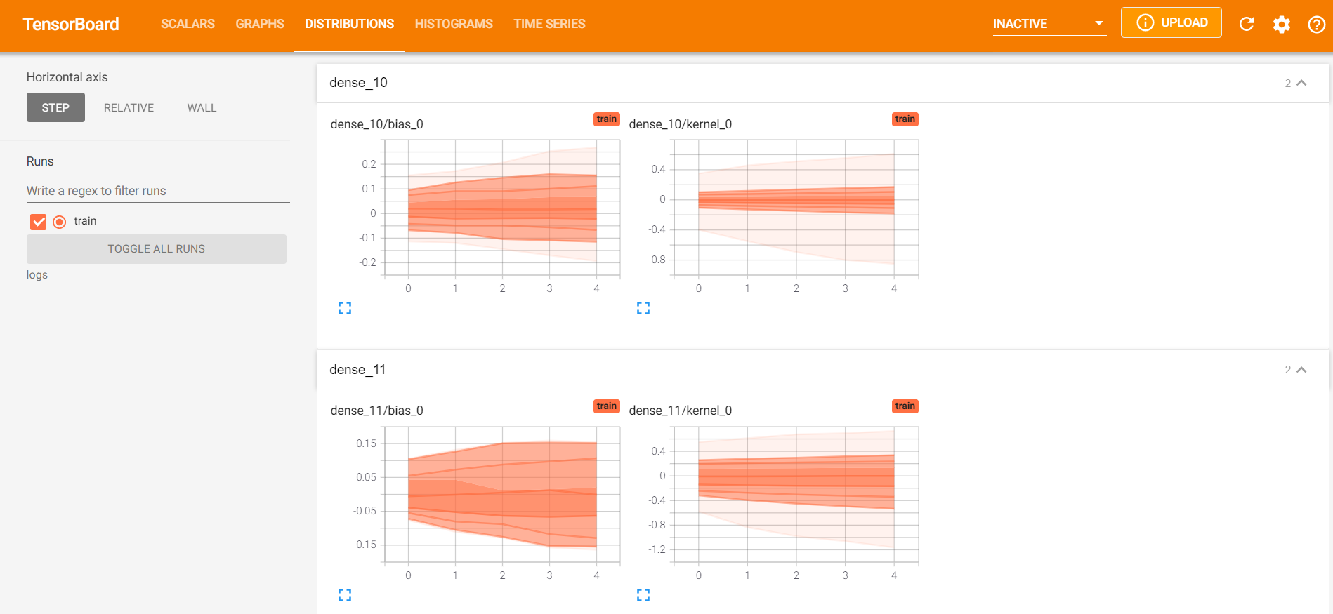
Distribution
This section shows the change of weights and biases over the time period of training.
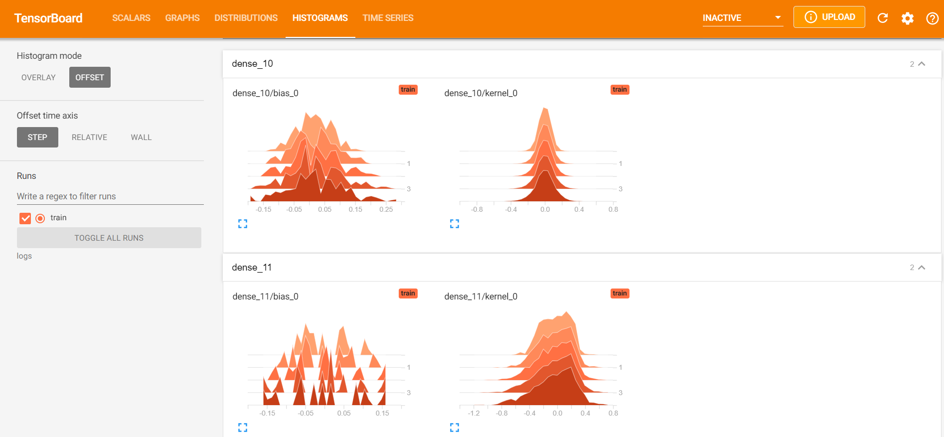
Histograms
This also shows the distribution of weights and bias over time in a 3D format.
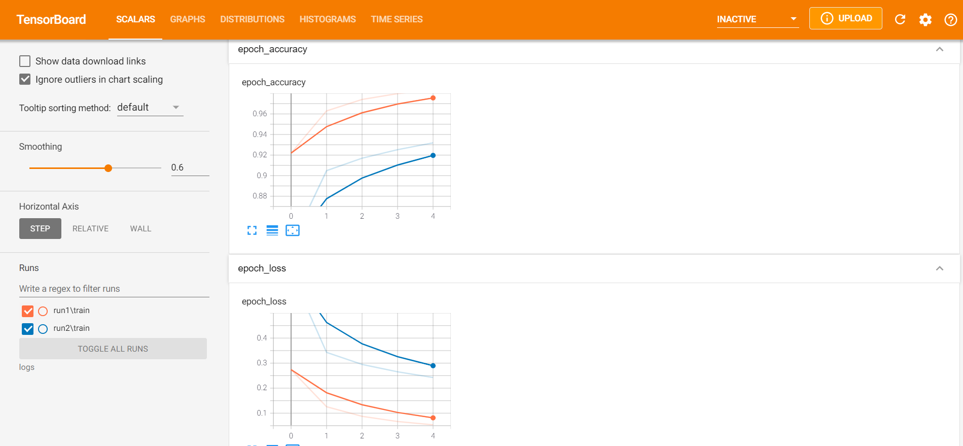
x) Comparing Different Models in TensorBoard
Creating a good Neural Network is not a straightforward job and requires multiple runs to experiment with various parameters. With TensorBoard, you can visualize the performance of all the model runs in the dashboard and compare them easily.
For this, we will create the logs of training in different subfolders inside the main folder. The below example will help you understand better.
In the first run, we create the Keras callback object of TensorBoard whose logs are going to be saved in the ‘run1’ folder inside the main logs folder.
tb_callback = tf.keras.callbacks.TensorBoard(log_dir="logs/run1", histogram_freq=1)
model.fit(X_train, y_train, epochs=5, callbacks=[tb_callback])
In the second run, we give the log path as run2 as shown below.
tb_callback = tf.keras.callbacks.TensorBoard(log_dir="logs/run2", histogram_freq=1)
model.fit(X_train, y_train, epochs=5, callbacks=[tb_callback])
Now when we see the TensorBoard dashboard, it will show information for both the runs in orange and blue lines for accuracy and loss graph.
Conclusion
Hope you found this article quite useful where we gave a small introductory tutorial on TensorBoard for beginners. We understood how to install and start the TensorBoard dashboard, along with various visualizations with the help of an example in Keras.

