Introduction
In this article, we will see an example of Tensorflow.js using the MNIST handwritten digit recognition dataset. For ease of understanding, this article is divided into three parts or files.
- The frontend – We will design the basic HTML file where we import Tensorflow.js and other required libraries.
- Fetching the dataset – We will use Google API to fetch the MNIST dataset.
- Model Building – We will use tensorflow.js to train & test our model. We will also visualize the results using tfvis library.
1. Frontend HTML file

Making a frontend HTML file
Open up an HTML file and initialize it as such (name it index.html)
<!DOCTYPE html>
<html>
<head>
  <meta charset="utf-8">
  <meta http-equiv="X-UA-Compatible" content="IE=edge">
  <meta name="viewport" content="width=device-width, initial-scale=1.0">
  <title>MLK TensorFlow.js Tutorial</title>
</head>
<body>
</body>
</html>
i) Importing Tensorflow.js
Remember that Tensorflow.js is a no-install machine learning framework. So, all you need to do is to define a script tag in the head tag of the HTML file above.
<script src="https://cdn.jsdelivr.net/npm/@tensorflow/[email protected]/dist/tf.min.js"></script>
ii) Importing tfjs-vis: Visualization library for Tensorflow.js
tfvis is a visualization library specifically made for visualizing training parameters of tensorflow.js models. It helps us to examine the training process and fine-tune the hyperparameters for making models.
Add this to the HTML header tag in order to import it.
<script src="https://cdn.jsdelivr.net/npm/@tensorflow/[email protected]/dist/tfjs-vis.umd.min.js"></script>
iii) The full HTML file
At this moment your HTML file will look like this –
<!DOCTYPE html>
<html>
<head>
  <meta charset="utf-8">
  <meta http-equiv="X-UA-Compatible" content="IE=edge">
  <meta name="viewport" content="width=device-width, initial-scale=1.0">
  <title>TensorFlow.js Tutorial</title>
  <!-- Import TensorFlow.js -->
  <script src="https://cdn.jsdelivr.net/npm/@tensorflow/[email protected]/dist/tf.min.js"></script>
  <!-- Import tfjs-vis -->
  <script src="https://cdn.jsdelivr.net/npm/@tensorflow/[email protected]/dist/tfjs-vis.umd.min.js"></script>
  <!-- Import the data file -->
  <script src="data.js" type="module"></script>
  <!-- Import the main script file -->
  <script src="script.js" type="module"></script>
</head>
<body>
</body>
</html>
2. Importing MNIST dataset in Tensorflow.js
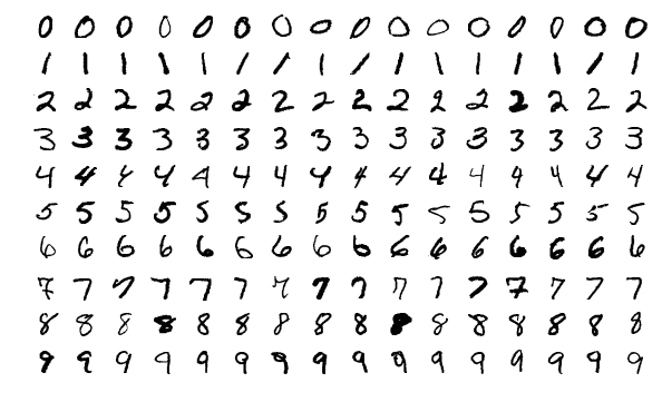
i) What is MNIST Dataset
The MNIST database is a large database of handwritten digits that is widely used for training and testing in the field of machine learning. It is commonly used as a benchmark dataset for testing various classification models. The MNIST dataset is an acronym that stands for the Modified National Institute of Standards and Technology. This dataset contains 65,000 small square 28×28 pixel grayscale images of handwritten single digits between 0 and 9.
ii) Fetching MNIST Dataset using Data.js
Data.js is a ready-to-use Javascript library provided by Tensorflowjs to fetch MNIST data and do operations with it.
Inside the data.js file, we can see that the images and labels of MNIST dataset is actually imported by using Google API.
const MNIST_IMAGES_SPRITE_PATH =
    'https://storage.googleapis.com/learnjs-data/model-builder/mnist_images.png';
const MNIST_LABELS_PATH =
    'https://storage.googleapis.com/learnjs-data/model-builder/mnist_labels_uint8';
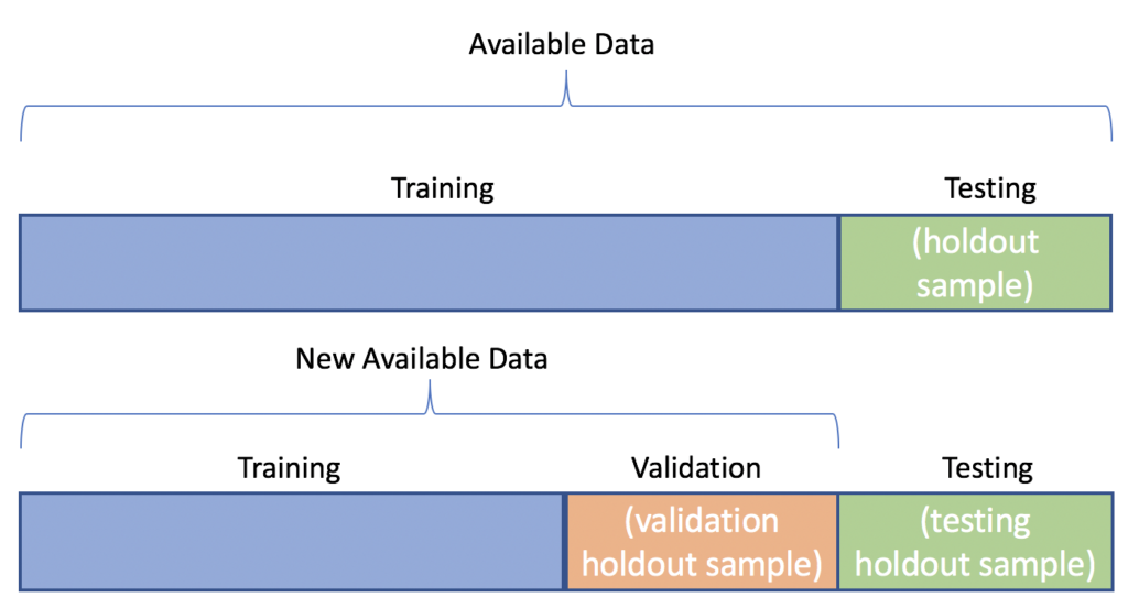
There are other parameters as well, which you can change as per your needs. For example, the below parameters signify that 6500 images will be imported which will be further divided into 55000 training and 10000 test images.
const NUM_DATASET_ELEMENTS = 65000;
const NUM_TRAIN_ELEMENTS = 55000;
iii) Important functions in Data.js
The data.js file consists of 4 functions:
- load(): This method makes an API call for the images, once they are loaded they are preprocessed (converted to uint8 data type). Then they are shuffled and divided into test and training datasets.
2. nextTrainBatch(): Fetches a specified no. of images from the training images dataset and returns them as an array.
3. nextTestBatch(): Fetches a specified no. of images from the testing images dataset and returns them as an array.
4. nextBatch(): It is an important function that directly fetches the entire data and passes it to the above two functions (nextTestBatch and nextTrainBatch) so that they can be returned as batches.
Import this file in our above HTML file’s header tag as well by adding:
<script src="data.js" type="module"></script>
You can find the full Pastebin for this file here
3. Model Building and Training
We will now build a new javascript file that will contain, the model definition, model training, model testing, and all the visualization functions.
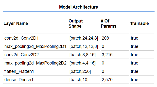
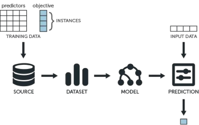
We will create the model as per the architecture shown below.
Note: Create a file script.js and import it into the HTML file like below. This entire section that we will discuss will be part of the script.js file.
<script src="script.js" type="module"></script>
i) Defining the model
Firstly we will be importing the data.js file from the second using the below lines.
import {MnistData} from './data.js';
Using the layers API of tensorflow.js we define the model type to be ‘sequential’ using the ‘tf.sequential()’ function. Next, we define the input parameters for the network layers i.e. image height, width, and channels along with the no of classes.
function getModel() {
    const model = tf.sequential();
    const IMAGE_WIDTH = 28;
    const IMAGE_HEIGHT = 28;
    const IMAGE_CHANNELS = 1;
    const NUM_OUTPUT_CLASSES = 10;}
Now, we start to add layers to our model using the ‘tf.add()’ function inside the ‘getModel’ function. We add a ‘conv2d’ layer with input dimensions equal to the width, height, no of channels along with ‘relu’ activation.
model.add(tf.layers.conv2d({inputShape: [IMAGE_WIDTH, IMAGE_HEIGHT, IMAGE_CHANNELS],kernelSize: 5,filters: 8,strides: 1,activation: 'relu',kernelInitializer: 'varianceScaling'}));
model.add(tf.layers.maxPooling2d({poolSize: [2, 2], strides: [2, 2]}));
// Repeat another conv2d + maxPooling stack.
model.add(tf.layers.conv2d({kernelSize: 5,filters: 16,strides: 1,activation: 'relu',kernelInitializer: 'varianceScaling'}));
model.add(tf.layers.maxPooling2d({poolSize: [2, 2], strides: [2, 2]}));
model.add(tf.layers.flatten());
model.add(tf.layers.dense({units: NUM_OUTPUT_CLASSES,kernelInitializer: 'varianceScaling',activation: 'softmax'}));
ii) Compiling the model
In order to compile the model, we use the ‘tf.compile’ function. This expects three parameters: a) An optimizer function(We will be using ‘adam’), b) the loss function(which will be categorical cross-entropy since there are more than two classes), and c) a performance metric (we will be choosing accuracy) so that the model strives towards the improvement of a certain metric.
const optimizer = tf.train.adam();
model.compile({optimizer: optimizer,loss: 'categoricalCrossentropy',metrics: ['accuracy'],});
Finally, we will be returning our compiled model inside the ‘getModel’ function. This will be the end of ‘getModel()’ function
return model;}
The ‘getModel’ function is now fully built, below is the complete function with all that we discussed in the above sections.
function getModel() {
    const model = tf.sequential();
    const IMAGE_WIDTH = 28;
    const IMAGE_HEIGHT = 28;
    const IMAGE_CHANNELS = 1;
   model.add(tf.layers.conv2d({inputShape: [IMAGE_WIDTH, IMAGE_HEIGHT, IMAGE_CHANNELS],kernelSize: 5,filters: 8,strides: 1,activation: 'relu',kernelInitializer: 'varianceScaling'}));

  // The MaxPooling layer acts as a sort of downsampling using max values in a region instead of averaging.
  model.add(tf.layers.maxPooling2d({poolSize: [2, 2], strides: [2, 2]}));

  // Repeat another conv2d + maxPooling stack.
  model.add(tf.layers.conv2d({kernelSize: 5,filters: 16,strides: 1,activation: 'relu',kernelInitializer: 'varianceScaling'}));
  model.add(tf.layers.maxPooling2d({poolSize: [2, 2], strides: [2, 2]}));

  // Now we flatten the output from the 2D filters into a 1D vector to prepare it for input into our last layer. This is common practice when feedinghigher dimensional data to a final classification output layer.
  model.add(tf.layers.flatten());

  // Our last layer is a dense layer which has 10 output units, one for each output class (i.e. 0, 1, 2, 3, 4, 5, 6, 7, 8, 9).
  const NUM_OUTPUT_CLASSES = 10;
  model.add(tf.layers.dense({units: NUM_OUTPUT_CLASSES,kernelInitializer: 'varianceScaling',activation: 'softmax'}));

  // Choose an optimizer, loss function and accuracy metric,
  // then compile and return the model
  const optimizer = tf.train.adam();
  model.compile({
    optimizer: optimizer,loss: 'categoricalCrossentropy',
    metrics: ['accuracy'],
});
iii) The Training Function
The training function will encompass multiple responsibilities such as defining the training metrics, fetch data to fit into the model, preprocess the data and finally fit it into the model. This will be an async function since we do not want to resume execution until and unless the training process is complete.
a) Parameters and callbacks
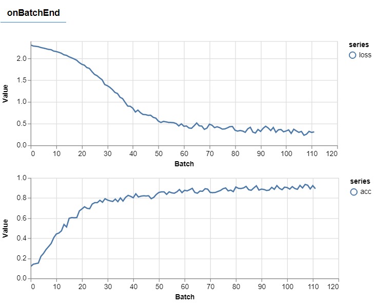
Below we are defining the 4 most important metrics (namely training and validation loss and training and validation accuracy) for visualization so that we can track them using the ‘tfvis’ visualization library.
Next, we pass the visualization function as a callback (using the ‘fitCallbacks’ function) so that after each epoch end the graph is updated and we can see the real-time performance of our model in the browser.
Finally, we define some model parameters:
- BATCH_SIZE: Refers to the no of units from the dataset to be shown to the model at once. We have chosen this value to be 512
- TRAIN_DATA_SIZE and TEST_DATA_SIZE: We will be training our model for 10 epochs thus the total no. of images in either set divided over 10 equal epochs will be 5500 and 1000 data points respectively.
async function train(model, data) {
    const metrics = ['loss', 'val_loss', 'acc', 'val_acc'];
    const container = {
      name: 'Model Training', tab: 'Model', styles: { height: '1000px' }};
    const fitCallbacks = tfvis.show.fitCallbacks(container, metrics);
    const BATCH_SIZE = 512;
    const TRAIN_DATA_SIZE = 5500;
    const TEST_DATA_SIZE = 1000;
The callback value for the model uses the TensorFlow visualization library and creates the graph similar to below during training:
b) Preprocessing and fetching functions
Thereafter we are using the ‘nextTestBatch’ and ‘nextTrainBatch’ to fetch data from the Google API and and put it in the const arrays (namely ‘trainXs’, ‘trainYs’ and ‘testXs’, ‘testYs’). But before that, the images are first reshaped into a size acceptable by our model i.e. a 4d array(no. of images, width, height, no. of color channels).
One can’t help but notice that all this is enclosed inside a ‘tf.tidy()’ function, this is so that the datasets are erased from memory when they are no longer in use.
const [trainXs, trainYs] = tf.tidy(() => {
      const d = data.nextTrainBatch(TRAIN_DATA_SIZE);
      return [
        d.xs.reshape([TRAIN_DATA_SIZE, 28, 28, 1]),d.labels];
    });
const [testXs, testYs] = tf.tidy(() => {
      const d = data.nextTestBatch(TEST_DATA_SIZE);
      return [
        d.xs.reshape([TEST_DATA_SIZE, 28, 28, 1]),d.labels];
    });
c) Fitting the model
The fit function is called to fit the dataset to the model with 512 as batch size and 10 epochs. This will be the end of ‘train()’ function.
return model.fit(trainXs, trainYs, {
      batchSize: BATCH_SIZE,
      validationData: [testXs, testYs],
      epochs: 10,
      shuffle: true,
      callbacks: fitCallbacks
    });}
This step marks the end of the ‘train’ function and complete function should look something like this:
  async function train(model, data) {
    const metrics = ['loss', 'val_loss', 'acc', 'val_acc'];
    const container = {
      name: 'Model Training', tab: 'Model', styles: { height: '1000px' }
    };
    const fitCallbacks = tfvis.show.fitCallbacks(container, metrics);
    const BATCH_SIZE = 512;
    const TRAIN_DATA_SIZE = 55000;
    const TEST_DATA_SIZE = 10000;
    const [trainXs, trainYs] = tf.tidy(() => {
      const d = data.nextTrainBatch(TRAIN_DATA_SIZE);
      return [
        d.xs.reshape([TRAIN_DATA_SIZE, 28, 28, 1]),d.labels];
    });

   const [testXs, testYs] = tf.tidy(() => {
      const d = data.nextTestBatch(TEST_DATA_SIZE);
      return [
        d.xs.reshape([TEST_DATA_SIZE, 28, 28, 1]),d.labels];
    });

   return model.fit(trainXs, trainYs, {
     batchSize: BATCH_SIZE,
     validationData: [testXs, testYs],
     epochs: 10,
     shuffle: true,
     callbacks: fitCallbacks
   });
}
iv) Getting Predictions
In order to get predictions, we use the ‘nextTestBatch’ function to fetch some images and store the true labels in the labels const. We preprocess them as before in order to get predictions. Then we use ‘.predict()’ functions to get predictions on the data and store them in the preds const.
const classNames = ['Zero', 'One', 'Two', 'Three', 'Four', 'Five', 'Six', 'Seven', 'Eight', 'Nine'];
function doPrediction(model, data, testDataSize = 500) {
  const IMAGE_WIDTH = 28;
  const IMAGE_HEIGHT = 28;
  const testData = data.nextTestBatch(testDataSize);
  const testxs = testData.xs.reshape([testDataSize, IMAGE_WIDTH, IMAGE_HEIGHT, 1]);
  const labels = testData.labels.argMax(-1);
  const preds = model.predict(testxs).argMax(-1);
  testxs.dispose();
  return [preds, labels];
}
v) Run Function
After defining all the nuts and bolts in the above sections we will now define a run() function that will trigger the entire process from loading data and training model when the page is loaded.
Inside the run() function we first load the data using the ‘data.js’ file. Next, we make a ‘model’ object and then call the ‘train()’ function with the ‘model’ and ‘data’ as parameters.
After that add an event listener is added which calls the ‘run()’ function every time the page is loaded or refreshed.
async function run() {
  const data = new MnistData();
  await data.load();
  const model = getModel();
  tfvis.show.modelSummary({name: 'Model Architecture', tab: 'Model'}, model);
  await train(model, data);
}
document.addEventListener('DOMContentLoaded', run);
vi) Visualizing the Training Process (Optional)
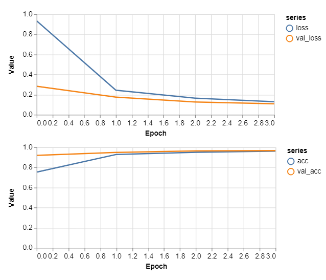
We use the prediction function to get the predictions and label array. Then we use the tensorflow.js visualization library to plot the accuracy in real-time.
async function showAccuracy(model, data) {
  const [preds, labels] = doPrediction(model, data);
  preds.print()
  const classAccuracy = await tfvis.metrics.perClassAccuracy(labels, preds);
  const container = {name: 'Accuracy', tab: 'Evaluation'};
  tfvis.show.perClassAccuracy(container, classAccuracy, classNames);
  labels.dispose();
}
await showAccuracy(model, data);
Conclusion
Hopefully, you liked the tutorial where saw the use of Tensorflow.js for building a model for the MNIST handwritten digit recognition dataset. You can download the soure code of this tutorial from the below links.
Links to source code files
- The HTML file(index.html)
- Data.js file(data.js)
- The training file(script.js)
Reference: Tensorflow.js Documentation