Introduction
In this article, we will go through the tutorial for Lane Detection in OpenCV Python using Hough Transform techniques. We will understand the problem statement of lane detection, what is Hough Transform, and its implementation functions in OpenCV Python with examples. Finally, we see the tutorial example of Lane detection on car dashcam video feed using Hough Transform in OpenCV Python.
What is Lane Detection?
As the name suggests, in the field of self-driving and autonomous vehicles lane detection refers to the identification or classification of lines on the road. A common use case is to confirm whether the car is driving in its own lane or has moved into another lane. While this is a simple use case the complex use case can be complete path identification for (self) driving to a particular destination by the autonomous vehicle.
The objective of Lane Detection is essentially to find the two straight lines of the lane, i.e. to find the straight lines in the image and this can be done using the Hough Transform technique.
What is Hough Transform?
Hough transform is a computer vision technique used for the purpose of feature isolation of particular shapes in images and videos i.e. it is a technique that can be successfully used to identify specific shapes in images – e.g. lines, circles, ellipses, etc. However, the trivial and original implementation of Hough Transform deals with detecting straight lines.
Hough Space
Let us assume we have a straight line and it can be represented as y=mx+c which is quite a common high school maths knowledge. But it can also be represented with the below equation
ρ = x*cos(θ) + y*sin(θ)
where –
- p (called rho) represents the distance from the origin
- θ (called theta) is the angle formed by the perpendicular line and horizontal axis measured in the counter-clockwise direction
This straight line can actually be represented with just two values (ρ, θ) and can be plotted in a space known as Hough Space.
As we can see in the illustration below, the straigh line that existed in the regular cartesian space is represented with just (ρ, θ) coordinates in the Hough Space.
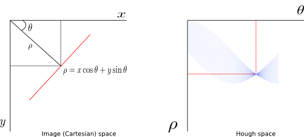
Every line in the original image is converted into the parametric form and represented using only these two values (ρ, θ) in the Hough Space. But why we need this Hough Space?
The intuition behind this is that while scanning the image, the same value of (ρ, θ) will occur many times for a straight line. The occurrences of (ρ, θ) can be accumulated as votes, and finally, when the scanning of the image is done, the (ρ, θ) value which got a high number of votes are identified as a line and can be reconstructed to its actual straight-line form to represent on the image.
To get the maximum performance, it is usually required to pass the image to the edge detector first before applying Hough Transform.
Hough Transform in OpenCV Python
It is quite easy to implement Hough Transform in OpenCV Python with the help of the built-in function cv2.HoughLines() whose syntax is shown below –
Syntax
lines = cv2.HoughLines(image,rho,theta,threshhold)
- image: Image src rho: Distance resolution of the accumulator (distance from the coordinate origin in the hough space)
- theta: Angle resolution of the accumulator(Line rotation in radians)
- threshold: Accumulator threshold parameter(Lines are only selected if they get votes equal to the threshold value))
Example of Hough Transform
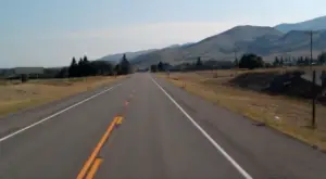
In this example, we will be applying Hough Transform with OpenCV Python function cv2.HoughLines() to detect lines on the following image –
Imports
import cv2
import numpy as np
img = cv2.imread('image.jpg')
gray = cv2.cvtColor(img,cv2.COLOR_BGR2GRAY)
edges = cv2.Canny(gray,50,150,apertureSize=3)
lines = cv2.HoughLines(edges,1,np.pi/180,200)
for line in lines:
   rho,theta=line[0]
   a=np.cos(theta)
   b=np.sin(theta)
   x0=a*rho
   y0=b*rho
   x1 = int(x0+1000*(-b))
   y1 = int(y0+1000*(a))
   x2 = int(x0-1000*(-b))
   y2 = int(y0-1000*(a))
   cv2.line(img,(x1,y1),(x2,y2),(255,0,255),2)
Line 1-3: According to the Hough transform algorithm the image needs to be converted to ‘GRAY’ colorspace (1) and sent for edge detection for which we use Canny function (2).
Line 4: We call the hough line transform function on the image. It returns an array of sub-arrays containing 2 elements each representing ρ and θ values for the line detected.
Line 5: Since the hough function returns an array of multiple subarrays, in order to loop through them we will initiate a for a loop.
Line 6-14: Computing the starting and endpoint of the lines detected using the ‘rho’ and ‘theta’ values returned to us by the hough function.
Line 15: Showing the lines on the original image using the ‘cv2.line’ function.
Output:
cv2.imshow("Lines",img)
cv2.waitKey(0)

Understanding Probabilistic Hough Transform
Probabilistic Hough Transform is an optimized version of Hough Transform. Firstly the lines that are predicted here are not unbounded (infinite) and second, they are enclosed in an area where the probability is maximum for these reasons the accuracy of the line detection process is more. (Returns 4 values for each sub-array, namely the start and endpoints)
Probabilistic Hough Transform in OpenCV Python
There is another function cv2.HoughLinesP() in OpenCV Python for Probabilistic Hough Transform who details are shown below –
Syntax
lines = cv2.HoughLinesP(image,rho,theta,threshold,minLineLength,maxLineGap)
- image: Image src rho: Distance resolution of the accumulator (distance from the coordinate origin in the hough space)
- theta: Angle resolution of the accumulator(Line rotation in radians)
- threshold: Accumulator threshold parameter(Lines are only selected if they get votes equal to the threshold value))
- minLineLength: Line segments shorter than this value are rejected
- maxLineGap: Max allowd gap between line segments to treat them as a single line
Example of Probabilistic Hough Transform
Again in this example, we will apply Probabilistic Hough Transform with OpenCV Python function cv2.HoughLinesP() to detect lines on the following image –
img = cv2.imread('image.jpg')
gray = cv2.cvtColor(img,cv2.COLOR_BGR2GRAY)
edges = cv2.Canny(gray,50,150,apertureSize=3)
lines = cv2.HoughLinesP(edges,1,np.pi/180,100,minLineLength=100,maxLineGap=40)
for line in lines:
     x1,y1,x2,y2=line[0]
     cv2.line(img,(x1,y1),(x2,y2),(0,255,0),2)
Line 1-3: Like in the above section, the probabilistic hough transform also expects a grayscale and edge detected image. So we perform those operations here.
Line 4: We call the probabilistic hough lines function HoughLinesP(). It returns an array that contains sub-arrays containing 4 values (x1,y1,x2,y2) each i.e. the starting and ending coordinates of the detected lines.
Line 5: Initiate a for loop in order to loop through the sub-arrays and show them one the original image.
Output:
cv2.imshow("Lines",img)
cv2.waitKey(0)

Tutorial – Lane Detection in OpenCV Python
As we discussed earlier, the main goal of the lane detection problem is to detect the two lines of the lane in the road. So to do lane detection in OpenCV Python we can just use the Hough Transform functions we learned above? No, it is not straightforward, let us understand why.
We have seen in the above sections that the Hough Transform function is able to detect lines in the image. But for lane detection, we need to make sure that we only detect lines present on the road itself and ignore the other probable lines that are present elsewhere in the image.
How are supposed to do that? This can be done using Masking.
Masking Function
By using a masking function we hide parts of our image so that the hough function only ‘sees’ the part of the image necessary for lane detection and perform line detection on that parts only.
The below implementation of the mask function will help as the first step to achieve our goal.
def roi(img,vertices):
    mask = np.zeros_like(img)
    cv2.fillPoly(mask,vertices,255)
    masked_image=cv2.bitwise_and(img,mask)
    return masked_image
Line 1: This function takes as input: i) An image (on which masking should be applied) and ii) An array containing coordinates of the vertices.
Line 2: Create a mask (with ‘0’ as pixel values) with a size equal to the image.
Line 3: Fill the mask with ‘1’ values inside the area formed by joining the coordinates present in the vertices array.
Line 4: The polygonal area formed by joining the points in the vertices array will be preserved in the image and the rest will be discarded. Perform the bitwise operation to achieve this operation.
Output:
#If this function is applied on an image independantly and with the following value of 'vertices' array
height = img.shape[0]
width = img.shape[1]
roi_vertices = [(0,height),(5*width/10,6*height/10),(width,height)]

Preprocessing Function
As we have learned before, the Hough Transform algorithm consists of converting an image into grayscale and passing it through an edge detection algorithm. Thus we make a preprocessing function that will help us preprocess each and every frame of a video or an image when required.
def preprocess(img):
    height = img.shape[0]
    width = img.shape[1]
    roi_vertices = [(0,height),(5*width/10,6*height/10),(width,height)]
    gray = cv2.cvtColor(img,cv2.COLOR_RGB2GRAY)
    canny = cv2.Canny(gray,100,150)
    cropped = roi(canny,np.array([roi_vertices],np.int32))
    return cropped
Line 1: This function takes an image as input and returns the preprocessed image.
Line 2-4: We will using the ‘roi’ function defined in the previous section so we first define the parameters of the vertices array that it takes as an argument.
Line 5-6: Convert the image to grayscale and apply canny edge detection.
Line 7: Apply the ‘roi’ function on the canny edge detected image.
Output:
Representation Function
It is quite evident that the probabilistic hough transform yields better results thus we will be using it for our lane detection purpose. As we discussed earlier it returns an array with sub-arrays containing coordinates of starting and endpoints of the detected lines. Thus we create a function that helps to represent the predicted lines.
def draw_hough_lines(img,lines):
    img = np.copy(img)
    blank_image = np.zeros((img.shape[0],img.shape[1],3),dtype=np.uint8)
    for line in lines:
        for x1,y1,x2,y2 in line:
            cv2.line(blank_image,(x1,y1),(x2,y2),(255,0,255),thickness=10)
    img = cv2.addWeighted(img,0.8,blank_image,1,0.0)
    return img
Line 2: We create a copy of the original image so as to not overwrite the original image.
Line 3: Initialize a blank image of the same size as our image.
Line 4-6: Loop through the ‘lines’ array to use the ‘cv2.line’ function to show each line on the ‘blank_image’.
Line 7: We use the ‘cv2.addWeighted’ function to perform blending of our ‘img’ and the ‘blank_image'(which now contains our lines) so that none of the images lose pixel values when superimposed.
Putting it all together
Next, we apply all the above functions together so that lane detection can be done on the frames of a video.
vid = cv2.VideoCapture('video.mp4')
while True:
ret,frame = vid.read()
if frame is None:
break
cropped= preprocess(frame)
lines = cv2.HoughLinesP(cropped,rho=6,threshold=60,theta=np.pi/180,minLineLength=50,maxLineGap=150,lines=np.array([]))
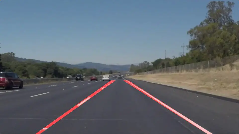
img = draw_hough_lines(frame,lines)
cv2.imshow('Lane detection',img)
if cv2.waitKey(1) & 0xFF == 27:
break
Line 1-2: Initialize the video object and a while loop to loop through the frames of a video.
Line 3-5: Fetch the video frame, if none break out of the loop.
Line 6: Call the processing function.
Line 7: Call the probabilistic hough lines function to generate an array that is filled with the coordinates of lines detected.
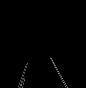
Line 8: Call the draw_hough_lines function so that the detected lines are visualized on the frame before showing it.
Line 9-11: If the user clicks the ‘escape’ button execution stops.
Results
Conclusion
Hope you liked this cool tutorial on lane detection in OpenCV Python using the Hough Transform algorithm. We understood the Hough Transform algorithm along with OpenCV python implementation and then used it for lane detection. You can certainly extend this tutorial into a full project with more creativity.