Tutorial – YOLOv5 Custom Object Detection in Colab

Introduction

In this article, we will go through the tutorial on how to use YOLOv5 for custom object detection in the Colab notebook. We will show you how to annotate our custom dataset, and set up your Google Colab environment for the training purpose.

We have already covered the basic introduction to YOLOv5 and how to use it in the following article that you may like to see to build the basics –

• Also Read – Introduction to YOLOv5 Object Detection with Tutorial

Tutorial Plan

Our tutorial to train custom YOLOv5 model for object detection will be divided into four main sections as below –

1. Annotate the images using LabelImg software
2. Environment Setup
3. Create training and data config files
4. Train our custom YOLOv5 object detector on the cloud
5. Inferencing our trained YOLOv5 custom object detection model

1. Data Annotation

In order to annotate our dataset, we will be using the LabelImg software. You can download it using this link for your machine.

Steps to Annotate:

1. Open LabelImg and select the ‘Open Dir’ option here, go to the directory where you have saved your images.

   

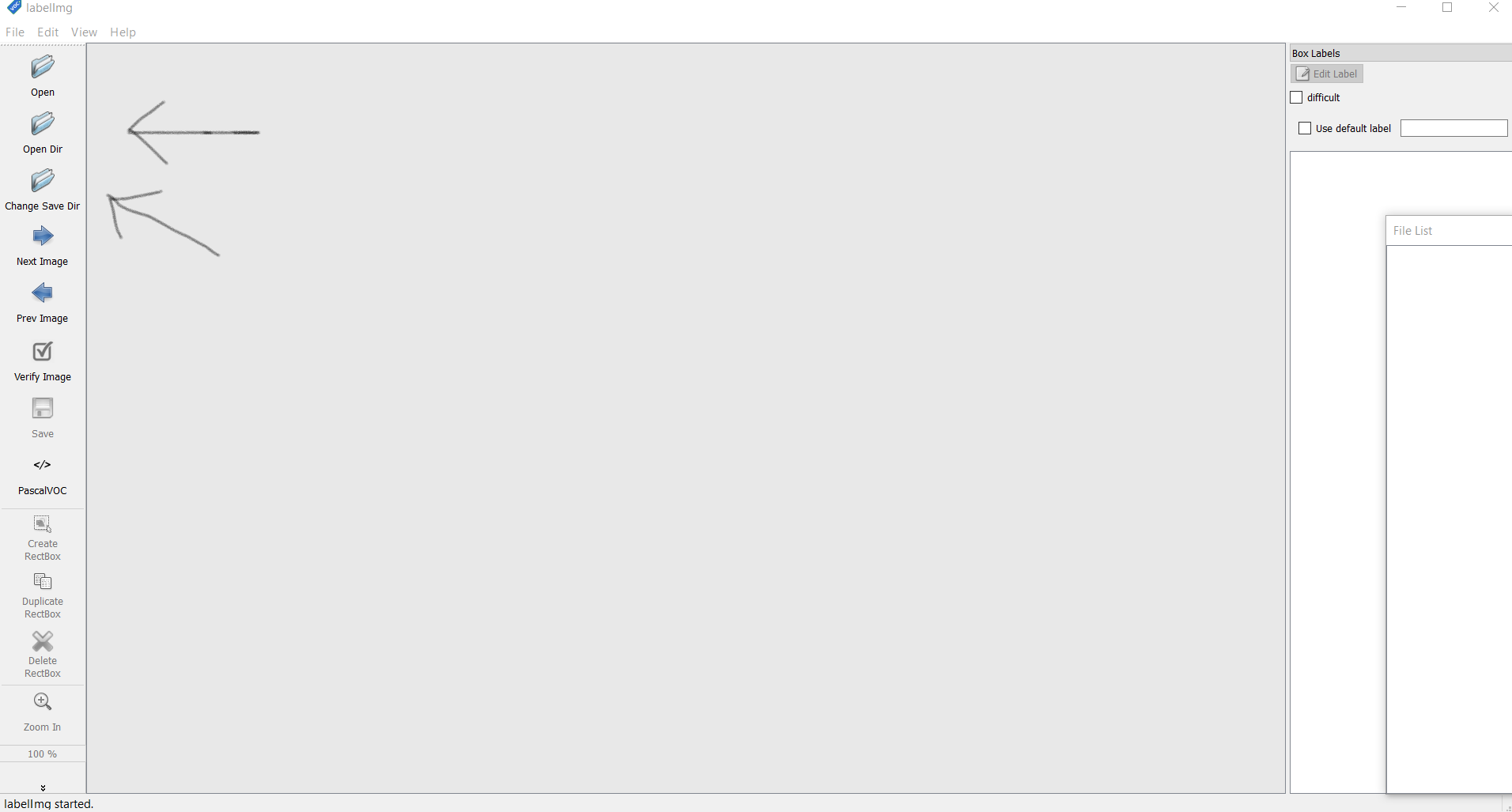
2. Next, select the ‘Change Save Dir’ and move to a directory where you want to save the annotations (text files). You can leave it just as it is and the images and text files will be saved in the same folder.

3. Change the pascalVOC format to YOLO by clicking on it.

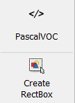
4. Now click the ‘Create Rectbox’ button and create a bounding a bounding box around the objects you want to detect. Next, add the name of the class the object belongs to.

This will create a classes.txt file which you have to delete. We delete it because the names of the classes will be defined in a separate file later.

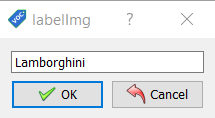
5. Click on ‘save'(in the sidebar) to save the annotation.

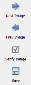
6. Click on ‘next’ to open the next image for annotation. Do this for all the images in the dataset.

7. Divide the dataset into two parts i.e. images and text documents separate. Further, divide them into train and validation sets. Look at the next section for more insight.

You should have a minimum of 250 images per class to reach a reasonable accuracy. The training and validation split can be 7:3(175:75). I personally collected and used 500 images and divided them into 400 training and 100 validation images.

2. Environment Setup

Uploading Data to Personal Drive

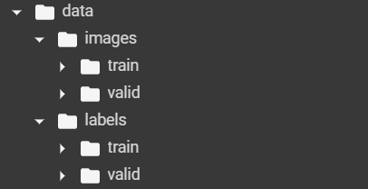
Create a data directory named ‘data’. The annotated data is supposed to be divided in such a way that the images and the annotations (text files) are separate. Further, each type of data is to be divided into two parts namely ‘train’ and ‘valid’ (which stands for training and validation data)

Your dataset directory should look something like this:

Setting Up Google Colab

Google Colab is an online environment similar to Jupiter notebook where you can train deep learning models on GPU. The free plan of Google Colab allows you to train the deep learning model for up to 12 hrs before the runtime disconnects.

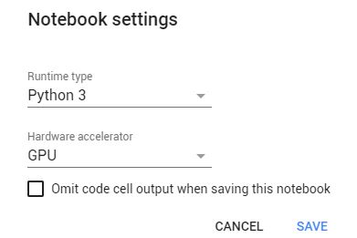
Setting GPU

By visiting the runtime section change the hardware accelerator to GPU.

Mounting Our Personal Drive

In order to use the dataset that we uploaded to the drive, we will mount our drive using the below code. (It will ask you to enter the authorization code that you can by clicking the link that will appear below)

from google.colab import drive
drive.mount('/content/drive')

Go to this URL in a browser: https://accounts.google.com/o/oauth2/auth?client_id=947318989803-6bn6qk8qdgf4n4g3pfee6491hc0brc4i.apps.googleusercontent.com&redirect_uri=urn%3aietf%3awg%3aoauth%3a2.0%3aoob&response_type=code&scope=email%20https%3a%2f%2fwww.googleapis.com%2fauth%2fdocs.test%20https%3a%2f%2fwww.googleapis.com%2fauth%2fdrive%20https%3a%2f%2fwww.googleapis.com%2fauth%2fdrive.photos.readonly%20https%3a%2f%2fwww.googleapis.com%2fauth%2fpeopleapi.readonly

Enter your authorization code:
··········
Mounted at /content/gdrive

Cloning The YOLOv5 repository

We will now clone the YOLOv5 repository provided by Ultralytics in our Colab environment.

!git clone https://github.com/ultralytics/yolov5

Output:

Cloning into 'yolov5'... 
remote: Enumerating objects: 7207, done. 
remote: Counting objects: 100% (313/313), done. 
remote: Compressing objects: 100% (194/194), done. 
remote: Total 7207 (delta 191), reused 212 (delta 119), pack-reused 6894 
Receiving objects: 100% (7207/7207), 9.18 MiB | 20.71 MiB/s, done. 
Resolving deltas: 100% (4929/4929), done.

Installing Requirements

Install the required dependencies and libraries required to use YOLOv5.

!pip install -r yolov5/requirements.txt

3. Creating Configuration Files

i) Model Architecture Configuration File

The model architecture file contains info about the no. of classes the dataset and original model was trained on 80 classes. Thus we will be creating the model architecture file directly using python and changing the ‘nc’ parameter to the no. of classes in our custom dataset.

The rest of the architecture is the same as the YOLOv5 S version.

Most importantly the file also holds the value of pre-computed anchors (that help us to detect objects) along with the architecture of the backbone and neck of our model. Other parameters like the structure of layers, no of layers, values of hyperparameters, and filters are also defined in these files.

You can look at it here or use this file.

with open('new_train_yaml', 'w+') as file:
    file.write(
        """
        # parameters
        nc: 1  # number of classes
        depth_multiple: 0.33  # model depth multiple
        width_multiple: 0.50  # layer channel multiple

        # anchors
        anchors:
          - [10,13, 16,30, 33,23]  # P3/8
          - [30,61, 62,45, 59,119]  # P4/16
          - [116,90, 156,198, 373,326]  # P5/32

        # YOLOv5 backbone
        backbone:
          # [from, number, module, args]
          [[-1, 1, Focus, [64, 3]],  # 0-P1/2
           [-1, 1, Conv, [128, 3, 2]],  # 1-P2/4
           [-1, 3, BottleneckCSP, [128]],
           [-1, 1, Conv, [256, 3, 2]],  # 3-P3/8
           [-1, 9, BottleneckCSP, [256]],
           [-1, 1, Conv, [512, 3, 2]],  # 5-P4/16
           [-1, 9, BottleneckCSP, [512]],
           [-1, 1, Conv, [1024, 3, 2]],  # 7-P5/32
           [-1, 1, SPP, [1024, [5, 9, 13]]],
           [-1, 3, BottleneckCSP, [1024, False]],  # 9
          ]

        # YOLOv5 head
        head:
          [[-1, 1, Conv, [512, 1, 1]],
           [-1, 1, nn.Upsample, [None, 2, 'nearest']],
           [[-1, 6], 1, Concat, [1]],  # cat backbone P4
           [-1, 3, BottleneckCSP, [512, False]],  # 13

           [-1, 1, Conv, [256, 1, 1]],
           [-1, 1, nn.Upsample, [None, 2, 'nearest']],
           [[-1, 4], 1, Concat, [1]],  # cat backbone P3
           [-1, 3, BottleneckCSP, [256, False]],  # 17 (P3/8-small)

           [-1, 1, Conv, [256, 3, 2]],
           [[-1, 14], 1, Concat, [1]],  # cat head P4
           [-1, 3, BottleneckCSP, [512, False]],  # 20 (P4/16-medium)

           [-1, 1, Conv, [512, 3, 2]],
           [[-1, 10], 1, Concat, [1]],  # cat head P5
           [-1, 3, BottleneckCSP, [1024, False]],  # 23 (P5/32-large)

           [[17, 20, 23], 1, Detect, [nc, anchors]],  # Detect(P3, P4, P5)
          ]
        """
    )

ii) Training Configuration File

Similar to the last section we will now create a training configuration file. Like the name suggests it provides the path to training and validation datasets. The ‘train’ and ‘val’ param provide the path to datasets while ‘nc’ represents the no. of classes and ‘names’ represents the class names associated with the class values (according to zero index).

with open('new_data_yaml', 'w+') as file:
    file.write(
        """
        train: /content/drive/MyDrive/data/images/train
        val: /content/drive/MyDrive/data/images/valid

        nc: 1
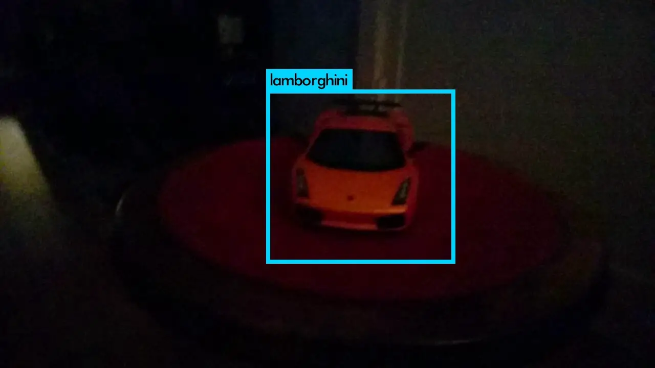
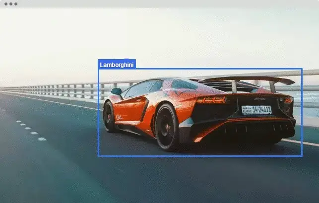
        names: ['Lamborghini']
        """
    )

4. Training Our Custom Object Detector Model

i) Training Command

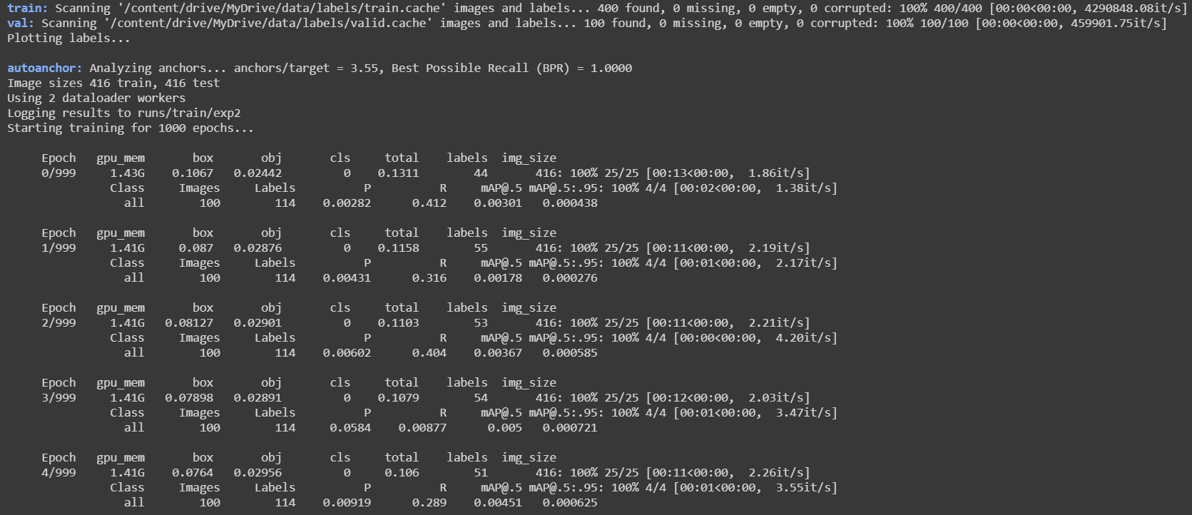
We will start the training process by running the following command that invokes ‘train.py’ file.

!python /content/yolov5/train.py --img 416 --batch 16 --epochs 500 --data /content/new_data_yaml --cfg /content/new_train_yaml

Parameters:

• –data: Path to the data configuration file
• –cfg: Path to the model architecture configuration file
• –img: Input image size
• –batch: Size of a batch (model weights are updated with each batch if you are on a personal machine use more no of batches so that PC doesn’t run out of memory).
• –epochs: No of epochs.

Output:

Results.png:

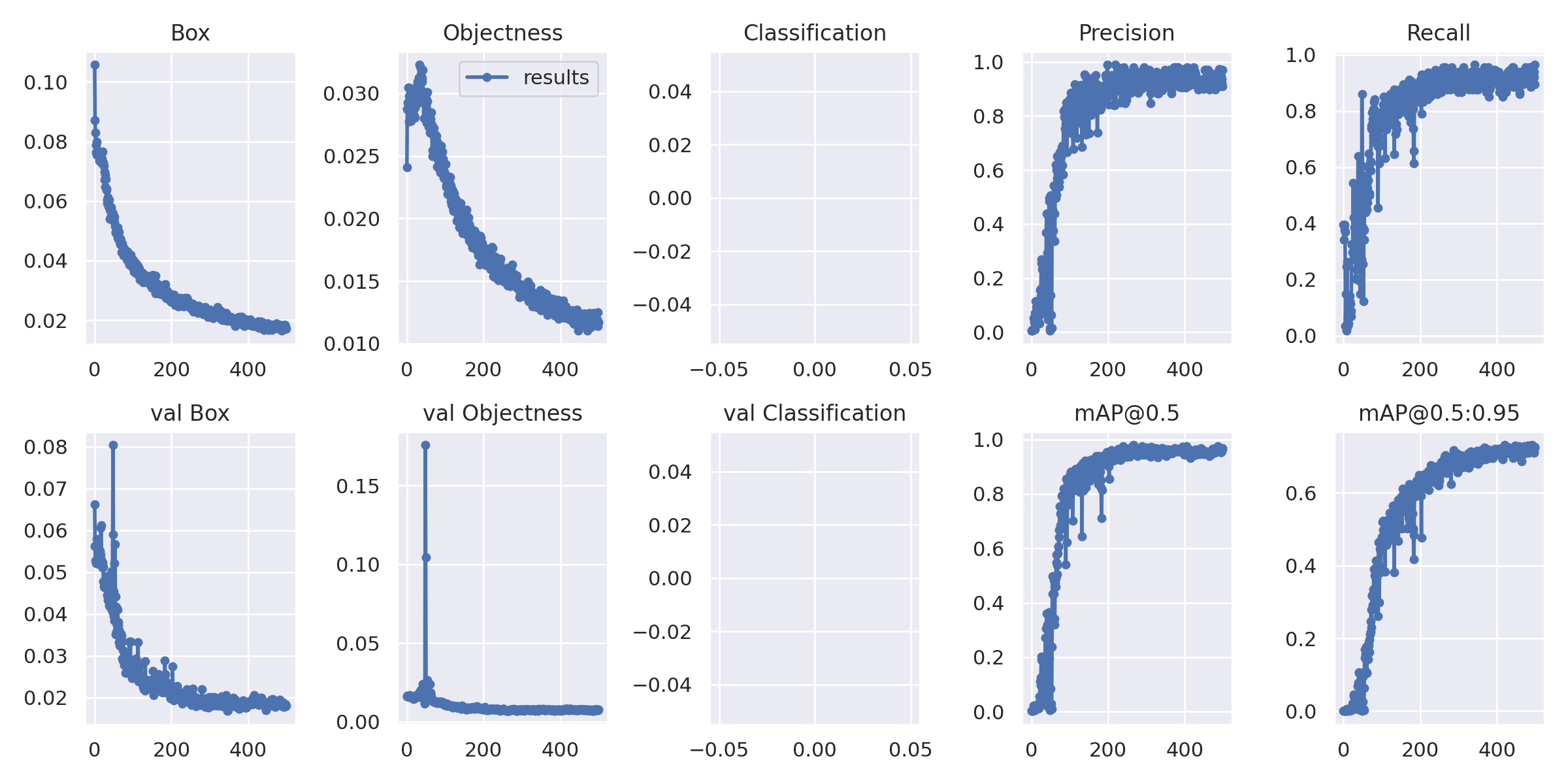
You may wonder why there is nothing in the classification graphs, it is because we only had one class thus classification was not required. In the case of multiple classes classification loss is also considered along with localization loss.

ii) Accessing the Custom Model

Output Directory

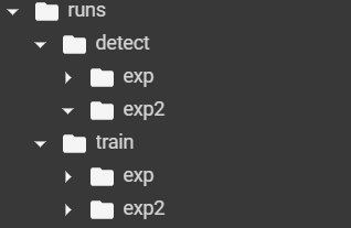
The very first time when the YOLOv5 model is called a folder called ‘runs’ is created that holds the outputs and info of each and every run. Each run is called an experiment and is created and saved in the following manner:(exp0, exp1, exp2, and so on). In case of inference ‘detection’ folder will be created whereas for training ‘train’ folder is created.

!ls /content/runs/train

Output:

exp

* Assuming that it is your first run the only folder in the ‘runs’ directory is ‘exp’.

We can take a look inside the ‘exp’ folder by using the following command.

!ls /content/runs/train/exp

Output: It will contain multiple graphs and visualization images that will provide an insight into the training process.

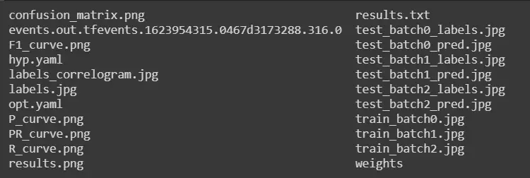
iii) Process and Data Visualization

Labels.jpg Image:

Confusion Matrix.png:

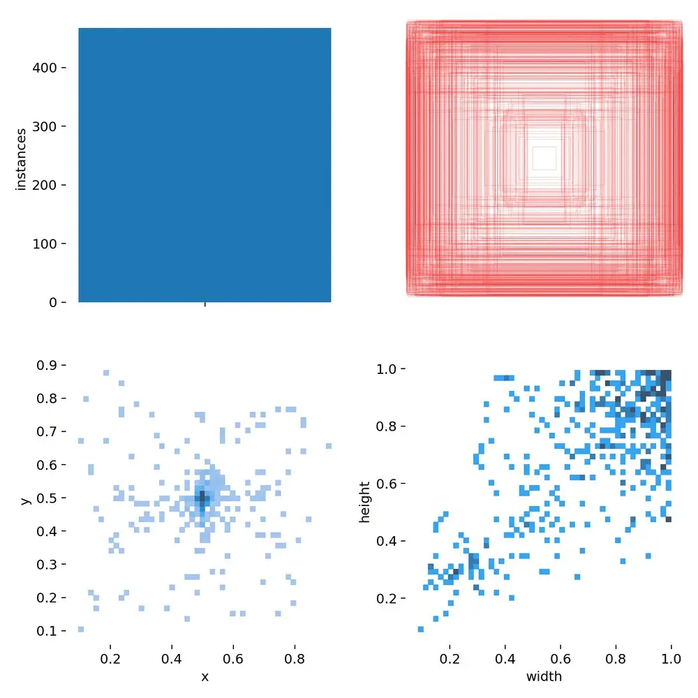
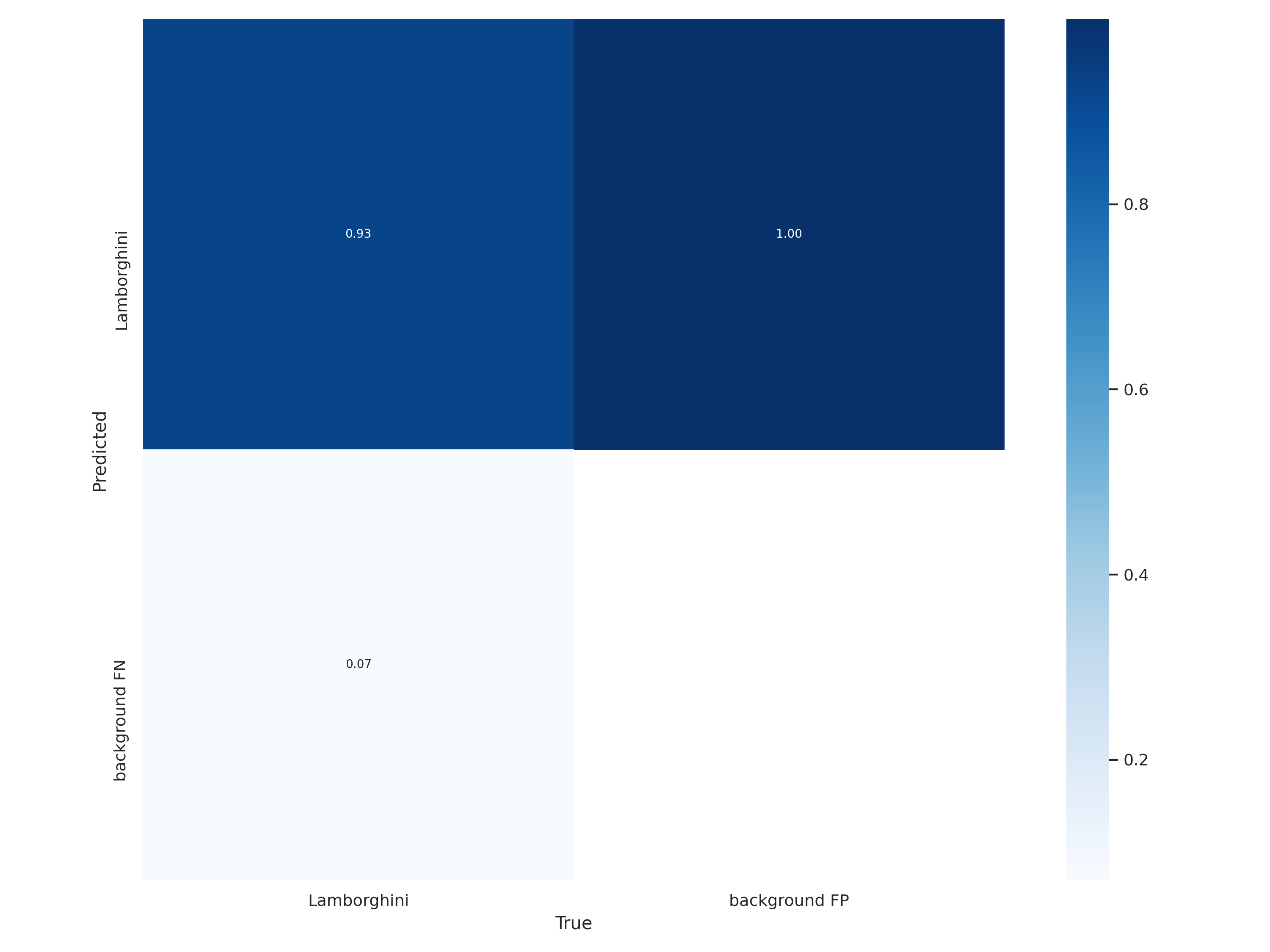
iv) Weights Directory

It has an additional ‘weights’ folder that holds the model weights that can be accessed using the following command:

!ls /content/runs/train/exp/weights

Output:

best.pt  last.pt

5. Inference using Custom YOLOv5 Object Detector

i) Inference Command

Run the ‘detect.py’ file to run inference on the custom dataset.

• –source: The path to the image to perform inference on.
• –weights: Weights file of the trained model.
• –img: The image will be resized to this value and then sent for detection.
• –conf: Minimum confidence value to consider a prediction as good.
• –save-txt: Flag parameters enables saving of text files containing the coordinates of bounding boxes.

!python /content/yolov5/detect.py --source testImage.jpg --weights '/conten/runs/train/exp/weights/last.pt' --img 416 --conf 0.5 --save-txt

Output:

Fusing layers... 
Model Summary: 232 layers, 7246518 parameters, 0 gradients, 16.8 GFLOPs 
image 1/1 testImage.jpg: 320x416 Done. (0.009s) 
Results saved to runs/detect/exp  
labels saved to runs/detect/exp/labels 
Done. (0.015s)

ii) Inference Results

YOLO automatically saves the annotated images (along with a text file containing the bounding box coordinates). You can find it in the YOLOv5 folder–> Inference folder–> Output folder.

!ls /runs/detect/exp

testImage.jpg labels

Conclusion

Coming to the end of this tutorial, hope you now know how to use YOLOv5 for custom object detection in Colab. Mind you custom training is the easiest part, the difficult part is the annotation of our custom dataset.