Python Sklearn Support Vector Machine (SVM) Tutorial with Example

Veer Kumar
Last Updated On February 6, 2022
Python

Table of Contents

Introduction

In this article, we will go through the tutorial for implementing the SVM (support vector machine) algorithm using the Sklearn (a.k.a Scikit Learn) library of Python. First, we will briefly understand the working of the SVM classifier. Then we will see an end-to-end project with a dataset to illustrate an example of SVM using the Sklearn module along with GridsearchCV for finding the best hyperparameters.

What is Support Vector Machine (SVM)

The Support Vector Machine Algorithm, better known as SVM is a supervised machine learning algorithm that finds applications in solving Classification and Regression problems.

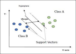
SVM makes use of extreme data points (vectors) in order to generate a hyperplane, these vectors/data points are called support vectors. The primary objective of the SVM algorithm is to create an optimal hyperplane with a maximum margin that can separate an n-dimensional space into distinct classes.

The below diagram illustrates the various aspects of the SVM –

Sklearn SVM (Support Vector Machine) — Source

Hyperplane: This is the decision boundary that separates two classes in n-dimensional space. The number of features present in our dataset set decides the number of hyperplanes. Suppose we have just two features, then the hyperplane will be a straight line, in the case of 3 features we get a 2-D plane.
Support Vectors: These data points affect the positioning of the hyperplane

Margin: Distance between a vector/data point and the hyperplane is called margin.
Maximum margin: Hyperplane with the maximum margin is called an optimal hyperplane.

Example of SVM in Python Sklearn

For creating an SVM classifier in Python, a function svm.SVC() is available in the Scikit-Learn package that is quite easy to use.

Let us understand its implementation with an end-to-end project example below where we will use medical data to predict if the person has heart disease or not.

i) Importing Required Libraries

We first import the libraries required to build our model.

In [2]:

#Import python packages
import numpy as np 
import pandas as pd 
import seaborn as sns
import matplotlib.pyplot as plt
from sklearn.model_selection import train_test_split # Import train_test_split function
from sklearn import svm #Import svm model
from sklearn import metrics #Import scikit-learn metrics module for accuracy calculation
from sklearn.metrics import confusion_matrix,roc_curve,roc_auc_score,accuracy_score, plot_confusion_matrix,classification_report

ii) Load Data

Next, we load the dataset in the CSV file into Pandas dataframes and verify if data is loading properly by using the head() function of dataframes.

In [3]:

df = pd.read_csv(r"C:\Users\Veer Kumar\Downloads\heart.csv")

In [4]:

df.head()

Out[4]:

	age	sex	cp	trestbps	chol	fbs	restecg	thalach	exang	oldpeak	slope	thal	target
0	63	1	3	145	233	1	0	150	0	2.3	0	1	1
1	37	1	2	130	250	0	1	187	0	3.5	0	2	1
2	41	0	1	130	204	0	0	172	0	1.4	2	2	1
3	56	1	1	120	236	0	1	178	0	0.8	2	2	1
4	57	0	0	120	354	0	1	163	1	0.6	2	2	1

iii) Details about Dataset

Our heart dataset has 303 rows and 14 columns. The significance of all the attributes present in the dataset is given below –

age: The person’s age in years

sex: The person’s sex (1 = male, 0 = female)
cp: The chest pain experienced (Value 1: typical angina, Value 2: atypical angina, Value 3: non-anginal pain, Value 4: asymptomatic)
trestbps: The person’s resting blood pressure (mm Hg on admission to the hospital) chol: The person’s cholesterol measurement in mg/dl

fbs: The person’s fasting blood sugar (> 120 mg/dl, 1 = true; 0 = false)
restecg: Resting electrocardiographic measurement (0 = normal, 1 = having ST-T wave abnormality, 2 = showing probable or definite left ventricular hypertrophy by Estes’ criteria)
thalach: The person’s maximum heart rate achieved

exang: Exercise induced angina (1 = yes; 0 = no)
oldpeak: ST depression induced by exercise relative to rest (‘ST’ relates to positions on the ECG plot. See more here)
slope: the slope of the peak exercise ST segment (Value 1: upsloping, Value 2: flat, Value 3: downsloping)

ca: The number of major vessels (0-3)
thal: A blood disorder called thalassemia (3 = normal; 6 = fixed defect; 7 = reversible defect)
target: Heart disease (0 = no, 1 = yes)

iv) Getting Summary Statistics of Dataset

We use the describe function() of pandas dataframes to quickly get a statistical glance at the dataset.

In [5]:

df.describe()

Out[5]:

	age	sex	cp	trestbps	chol	fbs	restecg	thalach	exang	oldpeak	slope	ca	thal	target
count	303.000000	303.000000	303.000000	303.000000	303.000000	303.000000	303.000000	303.000000	303.000000	303.000000	303.000000	303.000000	303.000000	303.000000
mean	54.366337	0.683168	0.966997	131.623762	246.264026	0.148515	0.528053	149.646865	0.326733	1.039604	1.399340	0.729373	2.313531	0.544554
std	9.082101	0.466011	1.032052	17.538143	51.830751	0.356198	0.525860	22.905161	0.469794	1.161075	0.616226	1.022606	0.612277	0.498835
min	29.000000	0.000000	0.000000	94.000000	126.000000	0.000000	0.000000	71.000000	0.000000	0.000000	0.000000	0.000000	0.000000	0.000000
25%	47.500000	0.000000	0.000000	120.000000	211.000000	0.000000	0.000000	133.500000	0.000000	0.000000	1.000000	0.000000	2.000000	0.000000
50%	55.000000	1.000000	1.000000	130.000000	240.000000	0.000000	1.000000	153.000000	0.000000	0.800000	1.000000	0.000000	2.000000	1.000000
75%	61.000000	1.000000	2.000000	140.000000	274.500000	0.000000	1.000000	166.000000	1.000000	1.600000	2.000000	1.000000	3.000000	1.000000
max	77.000000	1.000000	3.000000	200.000000	564.000000	1.000000	2.000000	202.000000	1.000000	6.200000	2.000000	4.000000	3.000000	1.000000

v) Visualize Data

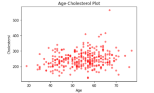
Here we visualize the relationship between the age of the patient and their cholesterol levels by using a scatter plot.

The plot indicates that the age groups 60 to 70 years old have slightly higher cholesterol levels as compared to other age groups. In addition to that, we also infer that ages below 40 mostly have cholesterol levels under 300 level.

In [7]:

df.plot(kind = 'scatter',x = 'age', y = 'chol',alpha = 0.5, color = 'red')
plt.xlabel('Age')
plt.ylabel('Cholesterol')
plt.title('Age-Cholesterol Plot')

Out[7]:

Text(0.5, 1.0, 'Age-Cholesterol Plot')

vi) Data Preprocessing

Here, we will separate the independent features and the target label.

In [8]:

#Separate Feature and Target Matrix
x = df.drop('target',axis = 1) 
y = df.target

vi) Splitting dataset into Train and Test Set

We split training and testing sets with the help of train_test_split() function

In [9]:

# Split dataset into training set and test set
# 70% training and 30% test
x_train, x_test, y_train, y_test = train_test_split(x, y, test_size=0.2,random_state=100)

vi) Creating and Training SVM Classifier

Here we create an SVM classifier that will be trained using the training data. Since our dataset is limited the K fold Cross-validation is a good method to estimate the performance of our model. Here, we use the GridSearchCV module in order to test a number of combinations of parameters that can optimize the performance of our model. For hyperparameter tuning we have 3 parameters to consider:

Kernel=rbf (radial basis function): kernel functions are used to map the original dataset (linear/nonlinear ) into a higher dimensional space with a view to making it a linear dataset.

C parameter: It is a hypermeter in SVM to control error. It acts as a penalty parameter, a small value of C will result in a larger margin separating the hyperplane. If we don’t want our training points to be misclassified, then we go for a large value of C, which will result in a smaller margin separating plane, but it can lead to an overfitting problem where the model may not generalize well on training data.
Gamma parameter: This will decide the curvature of the decision boundary, higher the gamma, the greater is the curvature of the decision boundary.

In [11]:

from sklearn.model_selection import GridSearchCV

#Create a svm Classifier and hyper parameter tuning 
ml = svm.SVC() 
  
# defining parameter range
param_grid = {'C': [ 1, 10, 100, 1000,10000], 
              'gamma': [1,0.1,0.01,0.001,0.0001],
              'kernel': ['rbf']} 
  
grid = GridSearchCV(ml, param_grid, refit = True, verbose = 1,cv=15)
  
# fitting the model for grid search
grid_search=grid.fit(x_train, y_train)

Out [11]:

Fitting 15 folds for each of 25 candidates, totalling 375 fits

[Parallel(n_jobs=1)]: Using backend SequentialBackend with 1 concurrent workers.
[Parallel(n_jobs=1)]: Done 375 out of 375 | elapsed:   11.7s finished

vii) Fetching Best Hyperparameters

Once training is complete, we can fetch the best hyperparameters from GridsearchCV and the corresponding accuracy score.

We can see that the values of C=100, gamma= 0.0001 produced the best results with an accuracy of 81.00%

In [12]:

print(grid_search.best_params_)

Out [12]:

{'C': 100, 'gamma': 0.0001, 'kernel': 'rbf'}

In [13]:

accuracy = grid_search.best_score_ *100
print("Accuracy for our training dataset with tuning is : {:.2f}%".format(accuracy) )

Out [13]:

Accuracy for our training dataset with tuning is : 81.00%

viii) Finding Test-Model Accuracy

Test model accuracy will tell us about how well our model generalized on the training data, on the basis of predicting values for unseen data. We can see that with an accuracy of 80.33% on test data our SVM classifier has indeed generalized well.

In [14]:

y_test_hat=grid.predict(x_test)
test_accuracy=accuracy_score(y_test,y_test_hat)*100
test_accuracy
print("Accuracy for our testing dataset with tuning is : {:.2f}%".format(test_accuracy) )

Out [14]:

Accuracy for our testing dataset with tuning is : 80.33%

ix) Plotting a Confusion Matrix

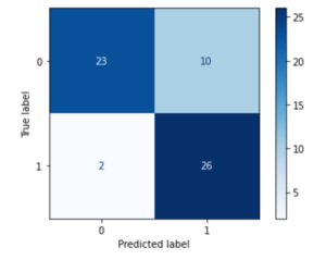
Finally, we evaluate the model using the testing data by using a confusion matrix to find out the number of true positives, true negatives, false positives, and false negatives.

In [15]:

confusion_matrix(y_test,y_test_hat)
disp=plot_confusion_matrix(grid, x_test, y_test,cmap=plt.cm.Blues)

Out[15]:

23 patients were predicted that they will have Heart Disease,the Prediction was CORRECT (True-Positive)
26 patients were predicted that they will NOT have Heart Disease,the Prediction was CORRECT (True-Negative)
10 patients were predicted that they will have Heart Disease but the Prediction was WRONG (False-Positive)

2 patients were predicted that they will NOT have Heart Disease but the Prediction was WRONG (False-Negative)

Also Read – Overfitting and Underfitting in Machine Learning – Animated Guide for Beginners

Conclusion

We hope you liked our tutorial and now better understand how to implement Support Vector Machines (SVM) using Sklearn(Scikit Learn) in Python. Here, we have illustrated an end-to-end example of using a dataset to build an SVM model in order to predict heart disease making use of the Sklearn svm.SVC() module.

Veer Kumar

I am passionate about Analytics and I am looking for opportunities to hone my current skills to gain prominence in the field of Data Science.
View all posts

Tags: machine learning, python, scikit learn, sklearn

2 Responses

Ritesh Patil says:

October 6, 2021 at 3:31 pm

A Good read ! Thank you !

Reply
1. MLK says:
  
  October 16, 2021 at 1:56 am
  
  Thank You Ritesh
  
  Reply