
Introduction
In this tutorial, we are going to see the Keras implementation of VGG16 architecture from scratch. VGG16 is a convolutional neural network architecture that was the runners up in the 2014 ImageNet challenge (ILSVR) with 92.7% top-5 test accuracy over a dataset of 14 million images belonging to 1000 classes. Although it finished runners up it went on to become quite a popular mainstream image classification model and is considered as one of the best image classification architecture.
In our Keras implementation of VGG16 architecture, we will use the well-known Dogs Vs Cats dataset from Kaggle. Moreover, we will use Google Colab to run our model on the GPU for fast training.
- Also Read – Learn Image Classification with Deep Neural Network using Keras
- Also Read – 7 Popular Image Classification Models in ImageNet Challenge (ILSVRC) Competition History
Dogs Vs Cats Kaggle Dataset
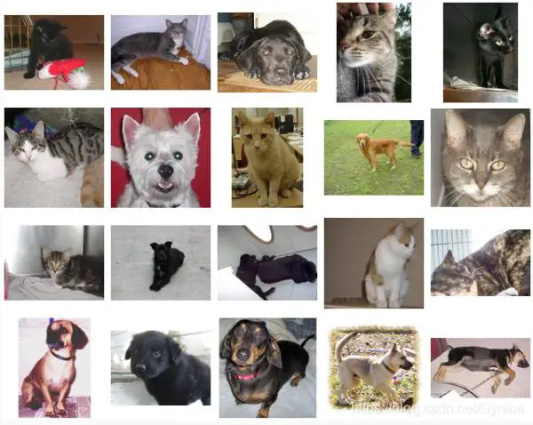
Dogs Vs Cats is a popular dataset from Kaggle which is often used for introductory lessons of Convolutional Neural Network. This dataset contains 25,000 images of dogs and cats for training a classification model.
Setting up Google Colab

We have uploaded the dataset on our google drive and before we can use it from Colab we need to mount the google drive directory on our runtime environment as shown below. This command will generate a URL on which you need to click, authenticate our Google drive account and copy the authorization key over here and press enter.
from google.colab import drive
drive.mount('/content/gdrive')
Now that we have set up the Google Colab let us start with the actual building of the Keras implementation of VGG16 image classification architecture.
VGG16 Keras Implementation
VGG16 Transfer Learning Approach
Deep Convolutional Neural networks may take days to train and require lots of computational resources. So to overcome this we will use Transfer Learning for implementing VGG16 with Keras.
Transfer learning is a technique whereby a deep neural network model that was trained earlier on a similar problem is leveraged to create a new model at hand. One or more layers from the already trained model are used in the new model. We will go through more details in a subsequent section below.
Importing libraries and setting up GPU
import cv2
import numpy as np
import os
from keras.preprocessing.image import ImageDataGenerator
from keras.layers import Dense,Flatten,Conv2D,Activation,Dropout
from keras import backend as K
import keras
from keras.models import Sequential, Model
from keras.models import load_model
from keras.optimizers import SGD
from keras.callbacks import EarlyStopping,ModelCheckpoint
from keras.layers import MaxPool2D
from google.colab.patches import cv2_imshow
K.tensorflow_backend._get_available_gpus()
Define training and testing path of dataset
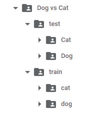
train_path="/content/gdrive/My Drive/datasets/train"
test_path="/content/gdrive/My Drive/datasets/test"
class_names=os.listdir(train_path)
class_names_test=os.listdir(test_path)
print(class_names)
print(class_names_test)
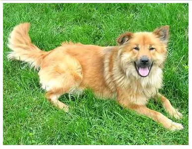
#Sample datasets images
image_dog=cv2.imread("/content/gdrive/My Drive/datasets/test/Dog/4.jpg")
cv2_imshow(image_dog)
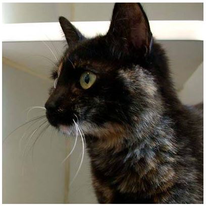
image_cat=cv2.imread("/content/gdrive/My Drive/datasets/test/Cat/5.jpg")
cv2_imshow(image_cat)
Preparation of datasets
We generally encountered problems where we try to load a dataset but there is not enough memory in your machine.
Keras provides the ImageDataGenerator class that defines the configuration for image data preparation and augmentation. The generator will progressively load the images in your dataset, allowing you to work with both small and very large datasets containing thousands or millions of images that may not fit into system memory.
train_datagen = ImageDataGenerator(zoom_range=0.15,width_shift_range=0.2,height_shift_range=0.2,shear_range=0.15)
test_datagen = ImageDataGenerator()
train_generator = train_datagen.flow_from_directory("/content/gdrive/My Drive/datasets/train",target_size=(224, 224),batch_size=32,shuffle=True,class_mode='binary')
test_generator = test_datagen.flow_from_directory("/content/gdrive/My Drive/datasets/test",target_size=(224,224),batch_size=32,shuffle=False,class_mode='binary')
VGG16 Architecture Overview
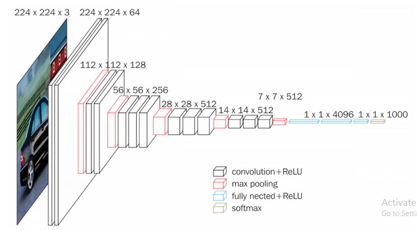
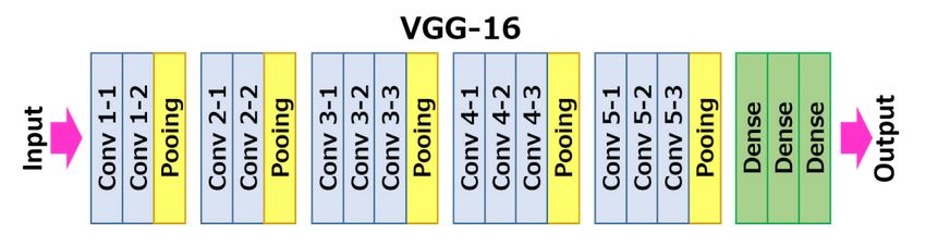
- VGG16 Architecture
- In VGG16 there are thirteen convolutional layers, five Max Pooling layers and three Dense layers which sum up to 21 layers but it has only sixteen weight layers i.e learnable parameters layer.
- It has convolution layers of 3×3 filter with a stride 1 and always used the same padding and maxpool layer of 2×2 filter of stride 2. It follows this arrangement of convolution and max pool layers consistently throughout the whole architecture.
- Conv-1 Layer has 64 number of filters ,Conv-2 has 128 filters,Conv-3 has 256 filters,Conv 4 and Conv 5 has 512 filters.
- Three Fully-Connected (FC) layers follow a stack of convolutional layers: the first two have 4096 channels each, the third performs 1000-way ILSVRC classification and thus contains 1000 channels (one for each class). The final layer is the soft-max layer.
- The input to Conv 1 layer is of fixed size 224 x 224 RGB image.
VGG16 Keras Implementation Design
Here we have defined a function and have implemented the VGG16 architecture using Keras framework. We have performed some changes in the dense layer. In our model, we have replaced it with our own three dense layers of dimension 256×128 with ReLU activation and finally 1 with sigmoid activation.
def VGG16():
    model = Sequential()
    model.add(Conv2D(input_shape=(224,224,3),filters=64,kernel_size=(3,3),padding="same", activation="relu"))
    model.add(Conv2D(filters=64,kernel_size=(3,3),padding="same", activation="relu"))
    model.add(MaxPool2D(pool_size=(2,2),strides=(2,2)))
    model.add(Conv2D(filters=128, kernel_size=(3,3), padding="same", activation="relu"))
    model.add(Conv2D(filters=128, kernel_size=(3,3), padding="same", activation="relu"))
    model.add(MaxPool2D(pool_size=(2,2),strides=(2,2)))
    model.add(Conv2D(filters=256, kernel_size=(3,3), padding="same", activation="relu"))
    model.add(Conv2D(filters=256, kernel_size=(3,3), padding="same", activation="relu"))
    model.add(Conv2D(filters=256, kernel_size=(3,3), padding="same", activation="relu"))
    model.add(MaxPool2D(pool_size=(2,2),strides=(2,2)))
    model.add(Conv2D(filters=512, kernel_size=(3,3), padding="same", activation="relu"))
    model.add(Conv2D(filters=512, kernel_size=(3,3), padding="same", activation="relu"))
    model.add(Conv2D(filters=512, kernel_size=(3,3), padding="same", activation="relu"))
    model.add(MaxPool2D(pool_size=(2,2),strides=(2,2),name='vgg16'))
    model.add(Flatten(name='flatten'))
    model.add(Dense(256, activation='relu', name='fc1'))
    model.add(Dense(128, activation='relu', name='fc2'))
    model.add(Dense(1, activation='sigmoid', name='output'))
    return model
model=VGG16()
model.summary()
As we discussed in the above section that we will use Transfer Learning for implementing VGG16 with Keras. So we will reuse the model weights from pre-trained models that were developed for standard computer vision benchmark datasets like ImageNet. We have downloaded pre-trained weights that do not have top layers weights. As you see above we have replaced the last three layers by our own layer and pre-trained weights do not contain the weights of newly three dense layers. So that is why we have to download pre-trained layer without top. (Link to download these weights are given at the bottom of the article)
Since we only have to initialize the weight to the last convolutional that is why we have called model and pass input as model input and output as the last convolutional block
Vgg16 = Model(inputs=model.input, outputs=model.get_layer('vgg16').output)
Now load the weights using the function load_weights of Keras
Vgg16.load_weights("/content/gdrive/My Drive/vgg16_weights_tf_dim_ordering_tf_kernels_notop.h5")
As we know that initial layers learn very general features and as we go higher up the network, the layers tend to learn patterns more specific to the task it is being trained on. So using these properties of the layer we want to keep the initial layers intact (freeze that layer) and retrain the later layers for our task. This is also termed as finetuning of a network.
The advantage of finetuning is that we do not have to train the entire layer from scratch and hence the amount of data required for training is not much either. Also, parameters that need to be updated are less and hence the amount of time required for training will also be less.
In Keras, each layer has a parameter called “trainable”. For freezing the weights of a particular layer, we should set this parameter to False, indicating that this layer should not be trained. After that, we go over each layer and select which layers we want to train.
In our case, we are freezing all the convolutional block of VGG16
for layer in Vgg16.layers:
    layer.trainable = False
Let us print all the layers in Vgg16 model. As you see here that up to last Maxpooling layer it is False which means that during training the parameters of these layers will not be updated. Whereas the last three layers have trainable parameter sets to true and hence during training the parameter of these layers gets updated.
for layer in model.layers:
    print(layer, layer.trainable)
We then compile the VGG16 using the compile function. This function expects three parameters: the optimizer, the loss function, and the metrics of performance. We are going to use stochastic gradient descent as an optimizer. Also since we are doing binary classification, we use binary_crossentropy as the choice for the loss function.
opt = SGD(lr=1e-4, momentum=0.9)
model.compile(loss="binary_crossentropy", optimizer=opt,metrics=["accuracy"])
[adrotate banner=”3″]
Early Stoping
So to overcome this problem the concept of Early Stoping is used.
In this technique, we can specify an arbitrarily large number of training epochs and stop training once the model performance stops improving on a hold out validation dataset. Keras supports the early stopping of training via a callback called EarlyStopping.
Below are various arguments in EarlyStopping.
- monitor – This allows us to specify the performance measure to monitor in order to end training.
- mode – It is used to specify whether the objective of the chosen metric is to increase maximize or to minimize.
- verbose – To discover the training epoch on which training was stopped, the “verbose” argument can be set to 1. Once stopped, the callback will print the epoch number.
- patience – The first sign of no further improvement may not be the best time to stop training. This is because the model may coast into a plateau of no improvement or even get slightly worse before getting much better. We can account for this by adding a delay to the trigger in terms of the number of epochs on which we would like to see no improvement. This can be done by setting the “patience” argument.
es=EarlyStopping(monitor='val_accuracy', mode='max', verbose=1, patience=20)
Model Check Point
The EarlyStopping callback will stop training once triggered, but the model at the end of training may not be the model with the best performance on the validation dataset.
An additional callback is required that will save the best model observed during training for later use. This is known as the ModelCheckpoint callback.
The ModelCheckpoint callback is flexible in the way it can be used, but in this case, we will use it only to save the best model observed during training as defined by a chosen performance measure on the validation dataset.
mc = ModelCheckpoint('/content/gdrive/My Drive/best_model.h5', monitor='val_accuracy', mode='max', save_best_only=True)
Training the Model
H = model.fit_generator(train_generator,validation_data=test_generator,epochs=100,verbose=1,callbacks=[mc,es])
model.load_weights("/content/gdrive/My Drive/best_model.h5")
Evaluating the model on test datasets
model.evaluate_generator(test_generator)
Serialize the Keras Model
It is the best practice of converting the model into JSON format to save it for the inference program in the future.
model_json = model.to_json()
with open("/content/gdrive/My Drive/model.json","w") as json_file:
  json_file.write(model_json)
Dogs Vs Cat Classification Inference Program
- We implemented the VGG16 model with Keras.
- We saved the best training weights of the model in a file for future use.
- We saved the model in JSON format for reusability.
- Load the model that we saved in JSON format earlier.
- Load the weight that we saved after training the model earlier.
- Compile the model.
- Load the image that we want to classify.
- Perform classification.
from keras.models import model_from_json
def predict_(image_path):
#Load the Model from Json File
json_file = open('/content/gdrive/My Drive/model.json', 'r')
model_json_c = json_file.read()
json_file.close()
model_c = model_from_json(model_json_c)
#Load the weights
model_c.load_weights("/content/gdrive/My Drive/best_model.h5")
#Compile the model
opt = SGD(lr=1e-4, momentum=0.9)
model_c.compile(loss="categorical_crossentropy", optimizer=opt,metrics=["accuracy"])
#load the image you want to classify
image = cv2.imread(image_path)
image = cv2.resize(image, (224,224))
cv2_imshow(image)
#predict the image
preds = model_c.predict(np.expand_dims(image, axis=0))[0]
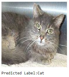
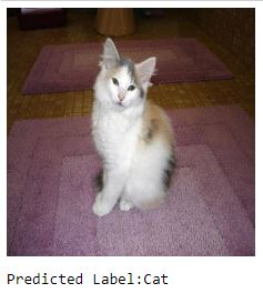
if preds==0:
print("Predicted Label:Cat")
else:
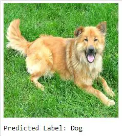
print("Predicted Label: Dog")
Perform Classification
predict_("/content/gdrive/My Drive/datasets/test/Dog/4.jpg")
predict_("/content/gdrive/My Drive/datasets/test/Cat/10.jpg")
predict_("/content/gdrive/My Drive/datasets/test/Cat/7.jpg")
Conclusion
Coming to the end of a long article, we hope you would now know how to implement VGG16 with Keras. We used Dog vs Cat dataset, but you can use just any dataset for creating your own VGG16 model with Keras.
Click Here is the link to download the weights
- Also Read – Learn Image Classification with Deep Neural Network using Keras
- Also Read – 7 Popular Image Classification Models in ImageNet Challenge (ILSVRC) Competition History

