Introduction
In this article, we will see the tutorial for doing word embeddings with the word2vec model in the Gensim library. We will first understand what is word embeddings and what is word2vec model. Then we will see its two types of architectures namely the Continuous Bag of Words (CBOW) model and Skip Gram model. Finally, we will explain how to use the pre-trained word2vec model and how to train a custom word2vec model in Gensim with your own text corpus. And as a bonus, we will also cover the visualization of our custom word2vec model.
What is Word Embeddings?
Machine learning and deep learning algorithms cannot work with text data directly, hence they need to be converted into numerical representations. In NLP, there are techniques like Bag of Words, Term Frequency, TF-IDF, to convert text into numeric vectors. However, these classical techniques do not represent the semantic relationship relationships between the texts in numeric form.
This is where word embedding comes into play. Word Embeddings are numeric vector representations of text that also maintain the semantic and contextual relationships within the words in the text corpus.
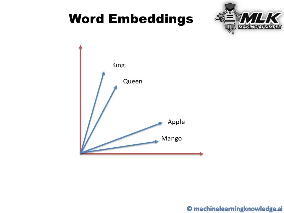
In such representation, the words that have stronger semantic relationships are closer to each other in the vector space. As you can see in the below example, the words Apple and Mango are close to each other as they both have many similar features of being fruit. Similarly, the words King and Queen are close to each other because they are similar in the royal context.
What is Word2Vec Model?
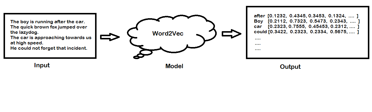
Word2vec is a popular technique for creating word embedding models by using neural network. The word2vec architectures were proposed by a team of researchers led by Tomas Mikolov at Google in 2013.
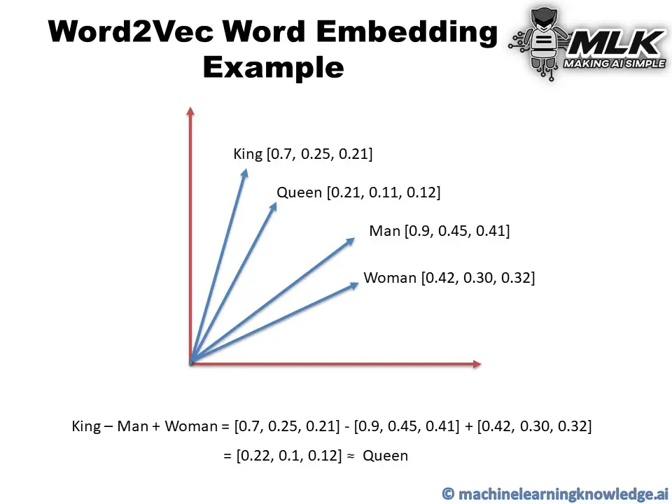
The word2vec model can create numeric vector representations of words from the training text corpus that maintains the semantic and syntactic relationship. A very famous example of how word2vec preserves the semantics is when you subtract the word Man from King and add Woman it gives you Queen as one of the closest results.
King – Man + Woman ≈ Queen
You may think about how we are doing addition or subtraction with words but do remember that these words are represented by numeric vectors in word2vec so when you apply subtraction and addition the resultant vector is closer to the vector representation of Queen.
In vector space, the word pair of King and Queen and the pair of Man and Woman have similar distances between them. This is another way putting that word2vec can draw the analogy that if Man is to Woman then Kind is to Queen!
The publicly released model of word2vec by Google consists of 300 features and the model is trained in the Google news dataset. The vocabulary size of the model is around 1.6 billion words. However, this might have taken a huge time for the model to be trained on but they have applied a method of simple subsampling approach to optimize the time.
Word2Vec Architecture
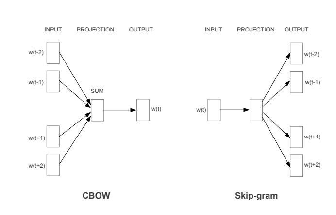
The paper proposed two word2vec architectures to create word embedding models – i) Continuous Bag of Words (CBOW) and ii) Skip-Gram.
i) Continuous Bag of Words (CBOW) Model
In the continuous bag of words architecture, the model predicts the current word from the surrounding context words. The length of the surrounding context word is the window size that is a tunable hyperparameter. The model can be trained by a single hidden layer neural network.
Once the neural network is trained, it results in the vector representation of the words in the training corpus. The size of the vector is also a hyperparameter that we can accordingly choose to produce the best possible results.
ii) Skip-Gram Model
In the skip-gram model, the neural network is trained to predict the surrounding context words given the current word as input. Here also the window size of the surrounding context words is a tunable parameter.
When the neural network is trained, it produces the vector representation of the words in the training corpus. Hera also the size of the vector is a hyperparameter that can be experimented with to produce the best results.
CBOW vs Skip-Gram Word2Vec Model
- CBOW model is trained by predicting the current word by giving the surrounding context words as input. Whereas the Skip-Gram model is trained by predicting the surrounding context words by providing the central word as input.
- CBOW model is faster to train as compared to the Skip-Gram model.
- CBOW model works well to represent the more frequently appearing words whereas Skip-Gram works better to represent less frequent rare words.
For details and information, you may refer to the original word2vec paper here.
Word2Vec using Gensim Library
Gensim is an open-source python library for natural language processing. Working with Word2Vec in Gensim is the easiest option for beginners due to its high-level API for training your own CBOW and SKip-Gram model or running a pre-trained word2vec model.
Installing Gensim Library
Let us install the Gensim library and its supporting library python-Levenshtein.
In[1]:
pip install gensim
pip install python-Levenshtein
In the below sections, we will show you how to run the pre-trained word2vec model in Gensim and then show you how to train your CBOW and SKip-Gram.
(All the examples are shown with Genism 4.0 and may not work with Genism 3.x version)
Working with Pretrained Word2Vec Model in Gensim
i) Download Pre-Trained Weights
We will use the pre-trained weights of word2vec that was trained on Google New corpus containing 3 billion words. This model consists of 300-dimensional vectors for 3 million words and phrases.
The weight can be downloaded from this link. It is a 1.5GB file so make sure you have enough space to save it.
ii) Load Libraries
We load the required Gensim libraries and modules as shown below –
In[2]:
import gensim
from gensim.models import Word2Vec,KeyedVectors
iii) Load Pre-Trained Weights
Next, we load our pre-trained weights by using the KeyedVectors.load_word2vec_format() module of Gensim. Make sure to give the right path of pre-trained weights in the first parameter. (In our case, it is saved in the current working directory)
In[3]:
model = KeyedVectors.load_word2vec_format('GoogleNews-vectors-negative300.bin.gz',binary=True,limit=100000)
iv) Checking Vectors of Words
We can check the numerical vector representation just like the below example where we have shown it for the word man.
In[4]:
vec = model['man']
print(vec)
Out[4]:
[ 0.32617188  0.13085938  0.03466797 -0.08300781  0.08984375 -0.04125977
 -0.19824219  0.00689697  0.14355469  0.0019455   0.02880859 -0.25
 -0.08398438 -0.15136719 -0.10205078  0.04077148 -0.09765625  0.05932617
  0.02978516 -0.10058594 -0.13085938  0.001297    0.02612305 -0.27148438
  0.06396484 -0.19140625 -0.078125    0.25976562  0.375      -0.04541016
  0.16210938  0.13671875 -0.06396484 -0.02062988 -0.09667969  0.25390625
  0.24804688 -0.12695312  0.07177734  0.3203125   0.03149414 -0.03857422
  0.21191406 -0.00811768  0.22265625 -0.13476562 -0.07617188  0.01049805
 -0.05175781  0.03808594 -0.13378906  0.125       0.0559082  -0.18261719
  0.08154297 -0.08447266 -0.07763672 -0.04345703  0.08105469 -0.01092529
  0.17480469  0.30664062 -0.04321289 -0.01416016  0.09082031 -0.00927734
 -0.03442383 -0.11523438  0.12451172 -0.0246582   0.08544922  0.14355469
 -0.27734375  0.03662109 -0.11035156  0.13085938 -0.01721191 -0.08056641
 -0.00708008 -0.02954102  0.30078125 -0.09033203  0.03149414 -0.18652344
 -0.11181641  0.10253906 -0.25976562 -0.02209473  0.16796875 -0.05322266
 -0.14550781 -0.01049805 -0.03039551 -0.03857422  0.11523438 -0.0062561
 -0.13964844  0.08007812  0.06103516 -0.15332031 -0.11132812 -0.14160156
  0.19824219 -0.06933594  0.29296875 -0.16015625  0.20898438  0.00041771
  0.01831055 -0.20214844  0.04760742  0.05810547 -0.0123291  -0.01989746
 -0.00364685 -0.0135498  -0.08251953 -0.03149414  0.00717163  0.20117188
  0.08300781 -0.0480957  -0.26367188 -0.09667969 -0.22558594 -0.09667969
  0.06494141 -0.02502441  0.08496094  0.03198242 -0.07568359 -0.25390625
 -0.11669922 -0.01446533 -0.16015625 -0.00701904 -0.05712891  0.02807617
 -0.09179688  0.25195312  0.24121094  0.06640625  0.12988281  0.17089844
 -0.13671875  0.1875     -0.10009766 -0.04199219 -0.12011719  0.00524902
  0.15625    -0.203125   -0.07128906 -0.06103516  0.01635742  0.18261719
  0.03588867 -0.04248047  0.16796875 -0.15039062 -0.16992188  0.01831055
  0.27734375 -0.01269531 -0.0390625  -0.15429688  0.18457031 -0.07910156
  0.09033203 -0.02709961  0.08251953  0.06738281 -0.16113281 -0.19628906
 -0.15234375 -0.04711914  0.04760742  0.05908203 -0.16894531 -0.14941406
  0.12988281  0.04321289  0.02624512 -0.1796875  -0.19628906  0.06445312
  0.08935547  0.1640625  -0.03808594 -0.09814453 -0.01483154  0.1875
  0.12792969  0.22753906  0.01818848 -0.07958984 -0.11376953 -0.06933594
 -0.15527344 -0.08105469 -0.09277344 -0.11328125 -0.15136719 -0.08007812
 -0.05126953 -0.15332031  0.11669922  0.06835938  0.0324707  -0.33984375
 -0.08154297 -0.08349609  0.04003906  0.04907227 -0.24121094 -0.13476562
 -0.05932617  0.12158203 -0.34179688  0.16503906  0.06176758 -0.18164062
  0.20117188 -0.07714844  0.1640625   0.00402832  0.30273438 -0.10009766
 -0.13671875 -0.05957031  0.0625     -0.21289062 -0.06542969  0.1796875
 -0.07763672 -0.01928711 -0.15039062 -0.00106049  0.03417969  0.03344727
  0.19335938  0.01965332 -0.19921875 -0.10644531  0.01525879  0.00927734
  0.01416016 -0.02392578  0.05883789  0.02368164  0.125       0.04760742
 -0.05566406  0.11572266  0.14746094  0.1015625  -0.07128906 -0.07714844
 -0.12597656  0.0291748   0.09521484 -0.12402344 -0.109375   -0.12890625
  0.16308594  0.28320312 -0.03149414  0.12304688 -0.23242188 -0.09375
 -0.12988281  0.0135498  -0.03881836 -0.08251953  0.00897217  0.16308594
  0.10546875 -0.13867188 -0.16503906 -0.03857422  0.10839844 -0.10498047
  0.06396484  0.38867188 -0.05981445 -0.0612793  -0.10449219 -0.16796875
  0.07177734  0.13964844  0.15527344 -0.03125    -0.20214844 -0.12988281
 -0.10058594 -0.06396484 -0.08349609 -0.30273438 -0.08007812  0.02099609]
iv) Most Similar Words
We can get the list of words similar to the given words by using the most_similar() API of Gensim.
In[5]:
model.most_similar('man')
Out[5]:
[(‘woman’, 0.7664012908935547),
(‘boy’, 0.6824871301651001),
(‘teenager’, 0.6586930155754089),
(‘teenage_girl’, 0.6147903203964233),
(‘girl’, 0.5921714305877686),
(‘robber’, 0.5585119128227234),
(‘teen_ager’, 0.5549196600914001),
(‘men’, 0.5489763021469116),
(‘guy’, 0.5420035123825073),
(‘person’, 0.5342026352882385)]
In[6]:
model.most_similar('PHP')
Out[6]:
[(‘ASP.NET’, 0.7275794744491577),
(‘Visual_Basic’, 0.6807329654693604),
(‘J2EE’, 0.6805503368377686),
(‘Drupal’, 0.6674476265907288),
(‘NET_Framework’, 0.6344218254089355),
(‘Perl’, 0.6339991688728333),
(‘MySQL’, 0.6315538883209229),
(‘AJAX’, 0.6286270618438721),
(‘plugins’, 0.6174636483192444),
(‘SQL’, 0.6123985052108765)]
v) Word Analogies
Let us now see the real working example of King-Man+Woman of word2vec in the below example. After doing this operation we use most_similar() API and can see Queen is at the top of the similarity list.
In[7]:
vec = model['king'] - model['man'] + model['women']
model.most_similar([vec])
Out[7]:
[(‘king’, 0.6478992700576782),
(‘queen’, 0.535493791103363),
(‘women’, 0.5233659148216248),
(‘kings’, 0.5162314772605896),
(‘queens’, 0.4995364248752594),
(‘princes’, 0.46233269572257996),
(‘monarch’, 0.45280295610427856),
(‘monarchy’, 0.4293173849582672),
(‘crown_prince’, 0.42302510142326355),
(‘womens’, 0.41756653785705566)]
Let us see another example, this time we do INR – India + England and amazingly the model returns the currency GBP in the most_similar results.
In[8]:
vec = model['INR'] - model ['India'] + model['England']
model.most_similar([vec])
Out[8]:
[(‘INR’, 0.6442341208457947),
(‘GBP’, 0.5040826797485352),
(‘England’, 0.44649264216423035),
(‘£’, 0.43340998888015747),
(‘Â_£’, 0.4307197630405426),
(‘£_#.##m’, 0.42561301589012146),
(‘GBP##’, 0.42464491724967957),
(‘stg’, 0.42324796319007874),
(‘EUR’, 0.418365478515625),
(‘€’, 0.4151178002357483)]
Training Custom Word2Vec Model in Gensim
i) Understanding Syntax of Word2Vec()
It is very easy to train custom wor2vec model in Gensim with your own text corpus by using Word2Vec() module of gensim.models by providing the following parameters –
- sentences: It is an iterable list of tokenized sentences that will serve as the corpus for training the model.
- min_count: If any word has a frequency below this, it will be ignored.
- workers: Number of CPU worker threads to be used for training the model.
- window: It is the maximum distance between the current and predicted word considered in the sentence during training.
- sg: This denotes the training algorithm. If sg=1 then skip-gram is used for training and if sg=0 then CBOW is used for training.
- epochs: Number of epochs for training.
These are just a few parameters that we are using, but there are many other parameters available for more flexibility. For full syntax check the Gensim documentation here.
ii) Dataset for Custom Training
For the training purpose, we are going to use the first book of the Harry Potter series – “The Philosopher’s Stone”. The text file version can be downloaded from this link.
iii) Loading Libraries
We will be loading the following libraries. TSNE and matplotlib are loaded to visualize the word embeddings of our custom word2vec model.
In[9]:
# For Data Preprocessing
import pandas as pd

# Gensim Libraries
import gensim
from gensim.models import Word2Vec,KeyedVectors

# For visualization of word2vec model
from sklearn.manifold import TSNE
import matplotlib.pyplot as plt
%matplotlib inline
iii) Loading of Dataset
Next, we load the dataset by using the pandas read_csv function.
In[10]:
df = pd.read_csv('HarryPotter.txt', delimiter = "\n",header=None)
df.columns = ['Line']
df
Out[10]:
| Line | |
|---|---|
| 0 | / |
| 1 | THE BOY WHO LIVED |
| 2 | Mr. and Mrs. Dursley, of number four, Privet D… |
| 3 | were proud to say that they were perfectly nor… |
| 4 | thank you very much. They were the last people… |
| … | … |
| 6757 | “Oh, I will,” said Harry, and they were surpri… |
| 6758 | the grin that was spreading over his face. “ T… |
| 6759 | know we’re not allowed to use magic at home. I’m |
| 6760 | going to have a lot of fun with Dudley this su… |
| 6761 | Page | 348 |
6762 rows × 1 columns
iv) Text Preprocessing
For preprocessing we are going to use gensim.utils.simple_preprocess that does the basic preprocessing by tokenizing the text corpus into a list of sentences and remove some stopwords and punctuations.
gensim.utils.simple_preprocess module is good for basic purposes but if you are going to create a serious model, we advise using other standard options and techniques for robust text cleaning and preprocessing.
In[11]:
preprocessed_text = df['Line'].apply(gensim.utils.simple_preprocess)
preprocessed_text
Out[11]:
0                                                      []
1                                  [the, boy, who, lived]
2       [mr, and, mrs, dursley, of, number, four, priv...
3       [were, proud, to, say, that, they, were, perfe...
4       [thank, you, very, much, they, were, the, last...
                              ...
6757    [oh, will, said, harry, and, they, were, surpr...
6758    [the, grin, that, was, spreading, over, his, f...
6759    [know, we, re, not, allowed, to, use, magic, a...
6760    [going, to, have, lot, of, fun, with, dudley, ...
6761                                               [page]
Name: Line, Length: 6762, dtype: object
v) Train CBOW Word2Vec Model
This is where we train the custom word2vec model with the CBOW technique. For this, we pass the value of sg=0 along with other parameters as shown below.
The value of other parameters is taken with experimentations and may not produce a good model since our goal is to explain the steps for training your own custom CBOW model. You may have to tune these hyperparameters to produce good results.
In[12]:
model_cbow = Word2Vec(sentences=preprocessed_text, sg=0, min_count=10, workers=4, window =3, epochs = 20)
Once the training is complete we can quickly check an example of finding the most similar words to “harry”. It actually does a good job to list out other character’s names that are close friends of Harry Potter. Is it not cool!
In[13]:
model_cbow.wv.most_similar("harry")
Out[13]:
[(‘ron’, 0.8734568953514099),
(‘neville’, 0.8471445441246033),
(‘hermione’, 0.7981335520744324),
(‘hagrid’, 0.7969962954521179),
(‘malfoy’, 0.7925101518630981),
(‘she’, 0.772059977054596),
(‘seamus’, 0.6930352449417114),
(‘quickly’, 0.692932665348053),
(‘he’, 0.691251814365387),
(‘suddenly’, 0.6806278228759766)]
v) Train Skip-Gram Word2Vec Model
For training word2vec with skip-gram technique, we pass the value of sg=1 along with other parameters as shown below. Again, these hyperparameters are just for experimentation and you may like to tune them for better results.
In[14]:
model_skipgram = Word2Vec(sentences =preprocessed_text, sg=1, min_count=10, workers=4, window =10, epochs = 20)
Again, once training is completed, we can check how this model works by finding the most similar words for “harry”. But this time we see the results are not as impressive as the one with CBOW.
In[15]:
model_skipgram.wv.most_similar("harry")
Out[15]:
[(‘goblin’, 0.5757830142974854),
(‘together’, 0.5725131630897522),
(‘shaking’, 0.5482161641120911),
(‘he’, 0.5105234980583191),
(‘working’, 0.5037856698036194),
(‘the’, 0.5015968084335327),
(‘page’, 0.4912668466567993),
(‘story’, 0.4897386431694031),
(‘furiously’, 0.4880291223526001),
(‘then’, 0.47639384865760803)]
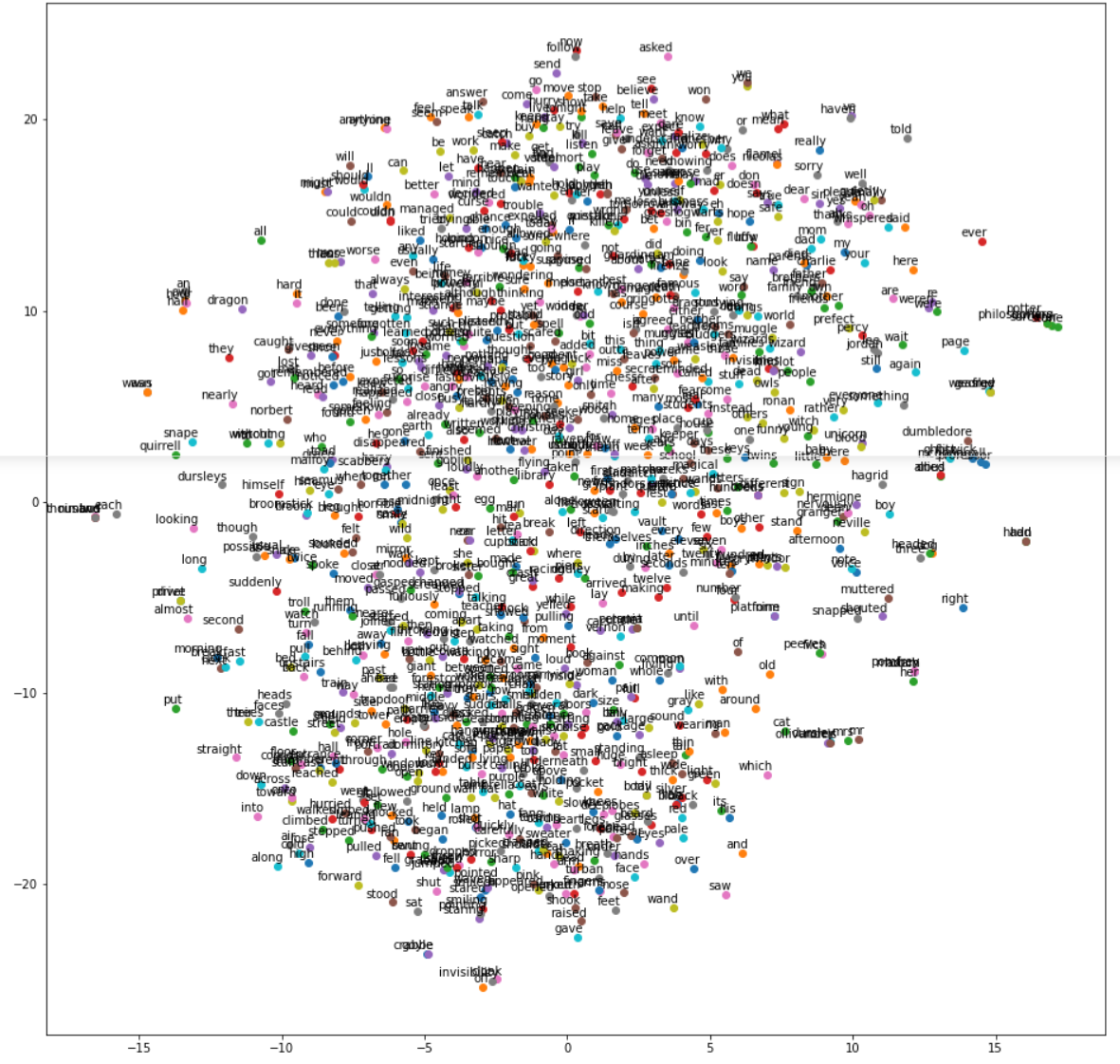
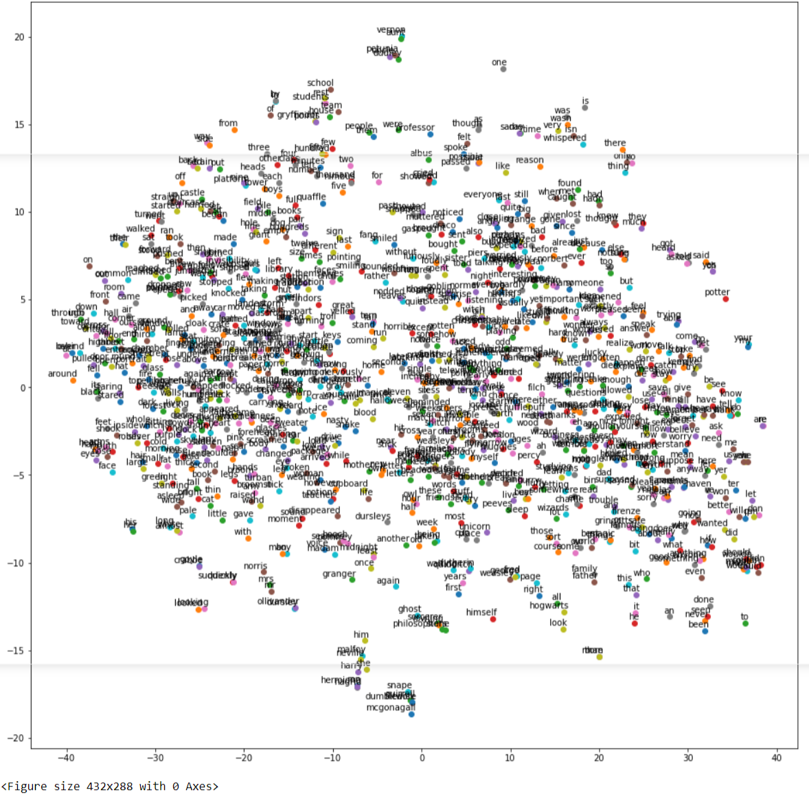
v) Visualizing Word Embeddings
The word embedding model created by wor2vec can be visualized by using Matplotlib and the TNSE module of Sklearn. The below code has been referenced from the Kaggle code by Jeff Delaney here and we have just modified the code to make it compatible with Gensim 4.0 version.
In[16]:
def tsne_plot(model):
    "Creates and TSNE model and plots it"
    labels = []
    tokens = []

    for word in model.wv.key_to_index:

        tokens.append(model.wv[word])
        labels.append(word)

    tsne_model = TSNE(perplexity=40, n_components=2, init='pca', n_iter=2500, random_state=23)
    new_values = tsne_model.fit_transform(tokens)

    x = []
    y = []
    for value in new_values:
        x.append(value[0])
        y.append(value[1])

    plt.figure(figsize=(16, 16))
    for i in range(len(x)):
        plt.scatter(x[i],y[i])
        plt.annotate(labels[i],
                     xy=(x[i], y[i]),
                     xytext=(5, 2),
                     textcoords='offset points',
                     ha='right',
                     va='bottom')
    plt.show()
a) Visualize Word Embeddings for CBOW
Let us visualize the word embeddings of our custom CBOW model by using the above custom function.
In[17]:
tsne_plot(model_cbow)
Out[17]:
b) Visualize Word Embeddings for Skip-Gram
Let us visualize the word embeddings of our custom Skip-Gram model by using the above custom function.
In[18]:
tsne_plot(model_skipgram)
Out[18]: