KNN Classifier in Sklearn using GridSearchCV with Example

Veer Kumar
Last Updated On September 4, 2021
Python

Table of Contents

Introduction

In this article, we will go through the tutorial for implementing the KNN classifier in Sklearn (a.k.a Scikit learn) library of Python. We will first understand the working of a KNN classifier followed by its characteristics. Then we will show you an end-to-end example of implementing the KNN classifier in Sklearn using GRidSearchCV for a classification problem in which we will classify genders as male or female based on certain facial features.

What is the KNN Algorithm in Machine Learning?

The KNN algorithm is a supervised learning algorithm where KNN stands for K-Nearest Neighbor. Usually, in most supervised learning algorithms, we train the model using training data set to create a model that generalizes well to predict unseen data.

But the KNN algorithm is a lazy algorithm that means there is absolutely no training phase involved. The algorithm just stores the initial training dataset and uses it at the time of the classification. (Hence it is a lazy execution)

At the same time, the KNN is a also non-parametric algorithm that signifies it does not assume any data distribution for it work properly.

How KNN Classification Works?

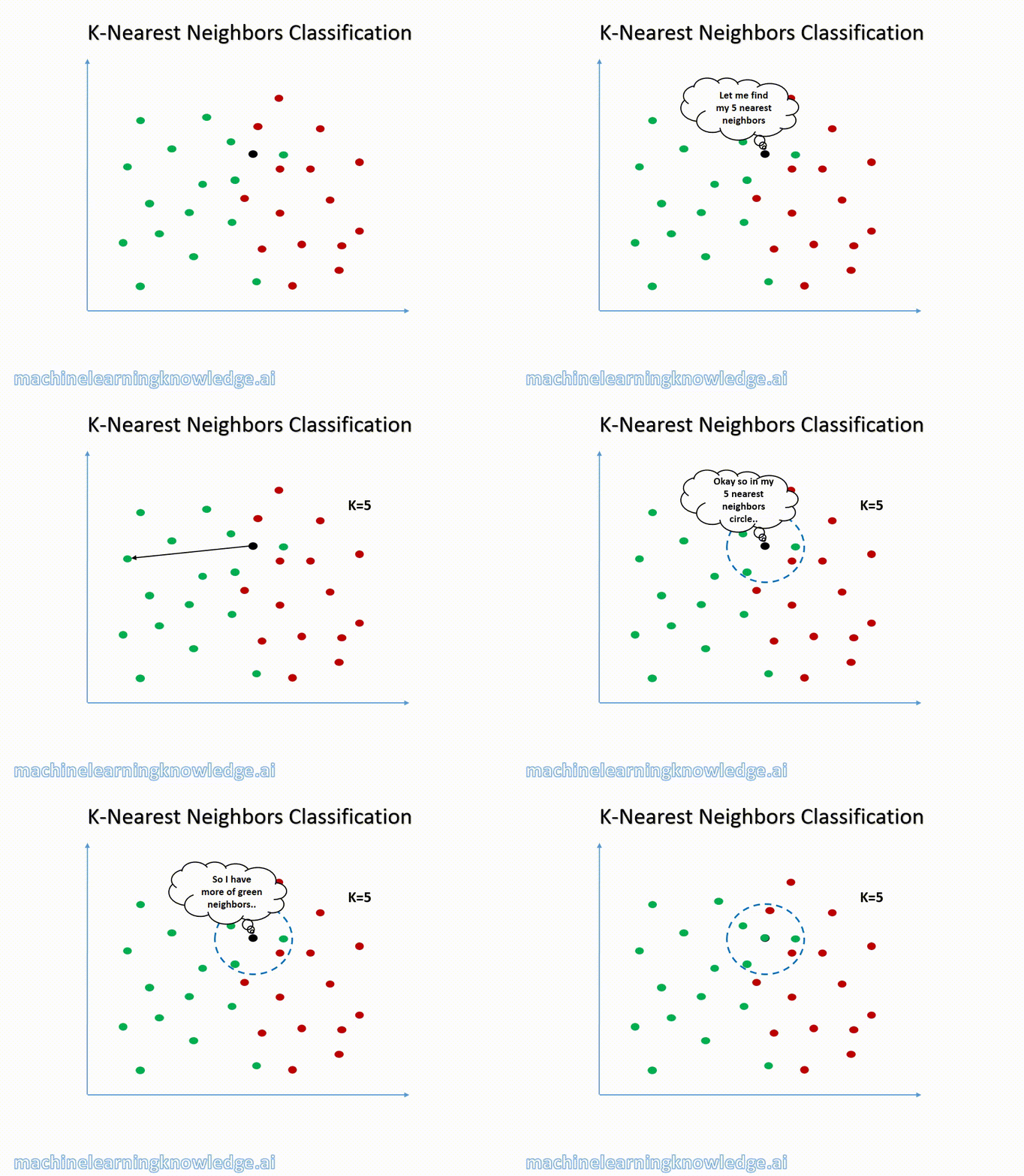
The KNN Classification algorithm itself is quite simple and intuitive. When a data point is provided to the algorithm, with a given value of K, it searches for the K nearest neighbors to that data point. The nearest neighbors are found by calculating the distance between the given data point and the data points in the initial dataset. You can use techniques like Euclidean distance, Manhattan distance, Cosine distance to calculate distance

Once K nearest neighbors are identified, the KNN algorithm next determines the majority of neighbors belong to which class. For example, if the majority of neighbors belong to class ‘Green’, then the given data point is also classified as class ‘Green’. The below illustration should make help you understand it better.

Points of consideration while implementing KNN algorithm

KNN is computationally expensive since it loads the entire dataset in the memory for classification. When the number of features of the dataset is very high it may suffer from curse of dimensionality and may perform poorly.
There is another aspect of the choice of the value of ‘K’ that can produce different results for different values of K. Hence hyperparameter tuning of K becomes an important role in producing a robust KNN classifier. In Sklearn we can use GridSearchCV to find the best value of K from the range of values. This will be shown in the example below.

Also Read – K Nearest Neighbor Classification – Animated Explanation for Beginners

KNN Classifier Example in SKlearn

The implementation of the KNN classifier in SKlearn can be done easily with the help of KNeighborsClassifier() module. In this example, we will use a gender dataset to classify as male or female based on facial features with the KNN classifier in Sklearn.

i) Importing Necessary Libraries

We first load the libraries required to build our model.

In [1]:

import pandas as pd
import numpy as np
import seaborn as sns
import matplotlib.pyplot as plt
from sklearn.metrics import confusion_matrix,plot_confusion_matrix

ii) About Gender Dataset

The gender dataset consists of 4981 rows and 7 features and one class label.

long_hair : it is 1 if he/she has long hair or 0 if he/she haven’t
forehead_width_cm : forehead width in cm

forehead_height_cm : forehead height in cm
nose_long : it is 1 if he/she has a long nose or 0 if he/she haven’t
nose_wide : it is 1 if he/she has a wide nose or 0 if he/she haven’t

lips_thin : it is 1 if he/she has thin lips or 0 if he/she haven’t
distance_nose_to_lip_long: it is 1 if there is a long distance between lips and nose or 0 if there isn’t this long distance between them
Gender(Target column): We will use the other 7 features of the dataset in order to make inferences and predictions regarding the gender of any given individual.

iii) Reading Dataset

We will read the dataset into Pandas dataframe and quickly browse through it.
Take high-level information about the dataset with info() function.
Check how many records are there for the two class labels Male and Female. We can see that is quite a balanced dataset.

In [2]:

df=pd.read_csv(r"C:\Users\Veer Kumar\Downloads\gender_classification_v7.csv")

In [3]:

df.head()

Out[3]:

	long_hair	forehead_width_cm	forehead_height_cm	nose_wide	nose_long	lips_thin	distance_nose_to_lip_long	gender
0	1	11.8	6.1	1	0	1	1	Male
1	0	14.0	5.4	0	0	1	0	Female
2	0	11.8	6.3	1	1	1	1	Male
3	0	14.4	6.1	0	1	1	1	Male
4	1	13.5	5.9	0	0	0	0	Female

In [4]:

df.info()

Out[4]:

<class 'pandas.core.frame.DataFrame'>
RangeIndex: 4981 entries, 0 to 4980
Data columns (total 8 columns):
 #   Column                     Non-Null Count  Dtype  
---  ------                     --------------  -----  
 0   long_hair                  4981 non-null   int64  
 1   forehead_width_cm          4981 non-null   float64
 2   forehead_height_cm         4981 non-null   float64
 3   nose_wide                  4981 non-null   int64  
 4   nose_long                  4981 non-null   int64  
 5   lips_thin                  4981 non-null   int64  
 6   distance_nose_to_lip_long  4981 non-null   int64  
 7   gender                     4981 non-null   object 
dtypes: float64(2), int64(5), object(1)
memory usage: 291.9+ KB

In [6]:

df['gender'].value_counts()

Out[6]:

Male      2492
Female    2489
Name: gender, dtype: int64

iv) Exploratory Data Analysis

After loading the dataset, we will do some exploratory data analysis to understand our data better.

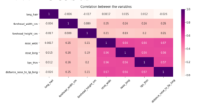
We first visualize the correlation between different features present in our data set. Then, we will use a line plot to understand strongly(positively) correlated features, followed by weekly correlated features, and ultimately will look at negatively correlated features.

In [9]:

#correlation matrix and the heatmap
plt.subplots(figsize=(12,5))
gender_correlation=df.corr()
sns.heatmap(gender_correlation,annot=True,cmap='RdPu')
plt.title('Correlation between the variables')
plt.xticks(rotation=45)

Out[9]:

(array([0.5, 1.5, 2.5, 3.5, 4.5, 5.5, 6.5]),
 [Text(0.5, 0, 'long_hair'),
  Text(1.5, 0, 'forehead_width_cm'),
  Text(2.5, 0, 'forehead_height_cm'),
  Text(3.5, 0, 'nose_wide'),
  Text(4.5, 0, 'nose_long'),
  Text(5.5, 0, 'lips_thin'),
  Text(6.5, 0, 'distance_nose_to_lip_long')])

In [10]:

sns.lineplot(data=df, x="distance_nose_to_lip_long", y="lips_thin")

Out[10]:

<AxesSubplot:xlabel='distance_nose_to_lip_long', ylabel='lips_thin'>

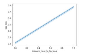
In the above lineplot, we observe that “lips_thin” and “distance_nose_to_lip_long” are positively correlated and they increase in almost a linear fashion.

In [11]:

sns.lineplot(data=df, x="forehead_width_cm", y="forehead_height_cm")

Out[11]:

<AxesSubplot:xlabel='forehead_width_cm', ylabel='forehead_height_cm'>

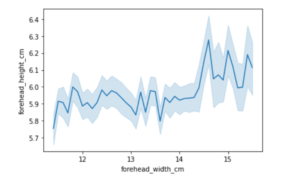
In the above line plot, we observe a haphazard and zigzag graph, this shows that “forehead_width_cm” and “forehead_height_cm” cannot be correlated, since they have a very small positive correlation, we cannot make any certain predictions by looking at this curve.

In [12]:

sns.lineplot(data=df, x="long_hair", y="forehead_width_cm")

Out[12]:

<AxesSubplot:xlabel='long_hair', ylabel='forehead_width_cm'>

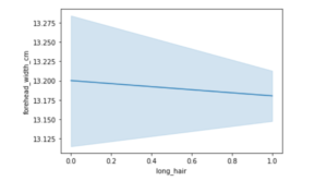
In this lineplot, presented above we see an example of negative correlation as can be observed from the negative slope when plotting quantities such as “long_hair” and “forehead_width_cm”.

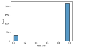
Here, we will compare an important feature called “nose_wide” that can be used to distinctly identify males from females or vice-versa.

In [13]:

males = df.query(" gender == 'Male' ")
males.groupby('nose_wide')['nose_wide'].describe()

Out[13]:

	count	mean	std	min	25%	50%	75%	max
nose_wide
0	316.0	0.0	0.0	0.0	0.0	0.0	0.0	0.0
1	2176.0	1.0	0.0	1.0	1.0	1.0	1.0	1.0

2176 males have a wide nose thaT means roughly 87% of males have this wide nose and just 316 males don’t have a wide nose.

In [14]:

sns.histplot(data = males , x = 'nose_wide')

Out[14]:

<AxesSubplot:xlabel='nose_wide', ylabel='Count'>

In [15]:

females = df.query(" gender == 'Female' ")
females.groupby('nose_wide')['nose_wide'].describe()

Out[15]:

	count	mean	std	min	25%	50%	75%	max
nose_wide
0	2202.0	0.0	0.0	0.0	0.0	0.0	0.0	0.0
1	287.0	1.0	0.0	1.0	1.0	1.0	1.0	1.0

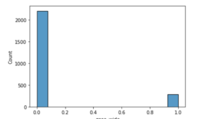
Here we see that 2202 females do not have a wide nose, while 287 have a wide nose. This means roughly 88% of women do not have a wide nose, which is a big difference from characteristics displayed by males for the same feature.

In [16]:

sns.histplot(data = females , x = 'nose_wide')

Out[16]:

<AxesSubplot:xlabel='nose_wide', ylabel='Count'>

v) Data Preprocessing

Here, we are separating the feature and target label into different dataframes x and y.

In [8]:

#preprocessing data
x = df.drop('gender', axis=1)
y = df['gender']

vi) Splitting Dataset into Training and Testing set

We split training and testing sets with the help of train_test_split() function.

In [17]:

#splitting the dataset
from sklearn.model_selection import train_test_split
# Split dataset into training set and test set
x_train, x_test, y_train, y_test = train_test_split(x, y, test_size=0.2,random_state=100)

In [18]:

from sklearn.neighbors import KNeighborsClassifier
from sklearn.metrics import accuracy_score, plot_confusion_matrix

vii) Model fitting with K-cross Validation and GridSearchCV

We first create a KNN classifier instance and then prepare a range of values of hyperparameter K from 1 to 31 that will be used by GridSearchCV to find the best value of K.

Furthermore, we set our cross-validation batch sizes cv = 10 and set scoring metrics as accuracy as our preference.

In [19]:

knn = KNeighborsClassifier()
from sklearn.model_selection import GridSearchCV
k_range = list(range(1, 31))
param_grid = dict(n_neighbors=k_range)
  
# defining parameter range
grid = GridSearchCV(knn, param_grid, cv=10, scoring='accuracy', return_train_score=False,verbose=1)
  
# fitting the model for grid search
grid_search=grid.fit(x_train, y_train)

Out[19]

Fitting 10 folds for each of 30 candidates, totalling 300 fits

[Parallel(n_jobs=1)]: Using backend SequentialBackend with 1 concurrent workers.
[Parallel(n_jobs=1)]: Done 300 out of 300 | elapsed:   22.6s finished

Once the model is fit, we can find the optimal parameter of K and the best score obtained through GridSearchCV. We can see that the best value of K is 26 and the corresponding accuracy is 97.64 %

In [24]:

print(grid_search.best_params_)

Out[24]

{'n_neighbors': 26}

In [20]:

accuracy = grid_search.best_score_ *100
print("Accuracy for our training dataset with tuning is : {:.2f}%".format(accuracy) )

Out[20]

Accuracy for our training dataset with tuning is : 97.64%

viii) Checking Accuracy on Test Data

Since now we have the best hyperparameter of K =26, this can be used to fit a KNN model and check its accuracy on the unseen test dataset.

In [21]:

knn = KNeighborsClassifier(n_neighbors=26)

knn.fit(X, y)

y_test_hat=knn.predict(x_test) 

test_accuracy=accuracy_score(y_test,y_test_hat)*100

print("Accuracy for our testing dataset with tuning is : {:.2f}%".format(test_accuracy) )

Out[21]

Accuracy for our testing dataset with tuning is : 96.49%

xi) Plotting a Confusion Matrix

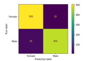
Now we evaluate the model using the testing data, for this purpose we set up a confusion matrix to help us in finding out true positives, true negatives, false positives, and false negatives.

In [22]:

plot_confusion_matrix(grid,x_train, y_train,values_format='d' )

Out[22]:

<sklearn.metrics._plot.confusion_matrix.ConfusionMatrixDisplay at 0x1ca1b2b0>

In [23]:

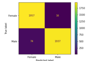
plot_confusion_matrix(grid,x_test, y_test,values_format='d' )

Out[23]:

<sklearn.metrics._plot.confusion_matrix.ConfusionMatrixDisplay at 0x1c9a7178>

Also Read – K Nearest Neighbor Classification – Animated Explanation for Beginners

Conclusion

We hope you liked our tutorial and now better understand how to implement the K-nearest neighbor (KNN) algorithm using Sklearn (Scikit Learn) in Python. Here, we have illustrated an end-to-end example of using a dataset to build a KNN model in order to classify our data points into their respective genders making use of the KNeighborsClassifier module.

Veer Kumar

I am passionate about Analytics and I am looking for opportunities to hone my current skills to gain prominence in the field of Data Science.
View all posts

Tags: machine learning, python, scikit learn, sklearn

One Response

Chima says:

May 10, 2022 at 4:22 am

You did a perfect job here. Thanks alot. very impressive

Reply