Introduction
The confusion matrix is rightly named so – it is really damn confusing !! It’s not only the beginners but sometimes even the regular ML or Data Science practitioners scratch their heads a bit when trying to calculate machine learning performance metrics with a “confusion matrix”.
To begin with, the confusion matrix is a method to interpret the results of the classification model in a better way. It further helps you to calculate some useful metrics that tells you about the performance of your machine learning model.
Come, let us take the confusion out of the confusion matrix.
Confusion Matrix – Building Step by Step Understanding
Let us take a very simple case of a binary classification that has only two possible outcomes True or False. To make it more clear let us consider an example of a binary classifier that scans the MRI images and predicts whether a person has cancer or not.
The outcomes predicted by classifier and the actual outcomes can only have the following four combinations –
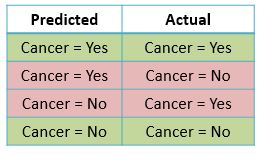
I hope so far so good, the above combination should not be difficult to understand. Now let us give a name to each of the four combinations –
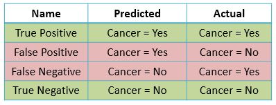
Let us elaborate on each of the four terms in detail.
True Positive
The model predicts that the patient is having cancer (positive) and indeed he has cancer (true prediction).
False Positive
The model predicts that the patient is having cancer (positive) but actually he is not having cancer (false prediction)
False Negative
The model predicts that the patient is not having cancer (negative) but he actually has cancer (false prediction).
True Negative
The model predicts that the patient is not having cancer (negative) and indeed he does not have cancer (true prediction).
Confusion Matrix
What we discussed above can be represented in the form of a matrix instead. This is how the Confusion Matrix looks like. Looks a bit simple now?
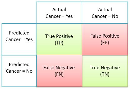
- TP = No. of True Positives from total predictions
- FP = No. of False Positives from total predictions
- FN = No. of False Negatives from total predictions
- TN = No. of True Negatives from total predictions
- TP+FP+FN+TN = Total no. of predictions
For the sake of better understanding let us represent this confusion matrix with real numbers. This will also serve us as a base to understand various machine learning performance metrics, which can be calculated using a confusion matrix.
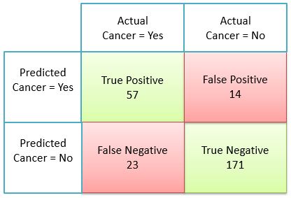
- 57= No. of True Positives from total predictions
- 14= No. of False Positives from total predictions
- 23= No. of False Negatives from total predictions
- 171= No. of True Negatives from total predictions
- 57+14+23+171 = 265 = Total no. of predictions
Performance Metrics
Once you have your confusion matrix ready, you can now use it to calculate various performance metrics to measure your classification models.
Let us understand the most popular metrics below.
Accuracy
Accuracy is a measure of the fraction of times the model predicted correctly (both true positive and true negative) out of total no. of predictions.
Accuracy = \(\frac { TP+TN }{ Total Predictions } \)
This is the simplest and very intuitive metrics. Let us consider the accuracy of the classifier in our example above.
Accuracy = \(\frac { 57+171 }{ 265} \) = 0.86
So this means our model can classify cancer and non cancer cases with 86% accuracy.
Accuracy can be misleading
Apparently, accuracy looks very obvious choice to measure the performance of the machine learning model. But there is a catch !!
Assume, that your machine model trains badly and only identifies negative scenarios
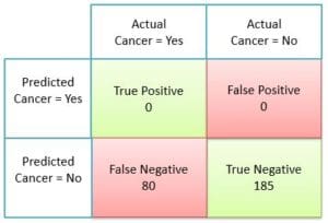
and miss to identify true positive completely. (This happens when there is a class imbalance in training data.)
So in our example, say the classifier completely misses to predict any case of cancer and marks all cases as non-cancer, this is how the confusion matrix will look like.
So the accuracy of our classifier will be
Accuracy = \(\frac { 185 }{ 265} \) = 0.70
So this is to say that the machine learning model which could not identify a single cancer case has an accuracy of 70% which is ridiculous.
I hope now you understand the problem of only relying on Accuracy for calculating the performance of the machine learning model.
This is why we have several other metrics to measure the performances of the machine learning model. Let us discuss them below.
Recall or Sensitivity or True Positive Rate
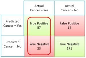
Recall is the fraction of times the model predicts positive cases correctly from the total number of actual positive cases.
Recall = \(\frac { TP }{ TP+FN } \)
Before you scratch your head, let me make you realize that TP+FN is the total number of actual positive cases that the classifier should have identified. But it could identify only TP cases and missed FN cases.
In our example, TP = 57 cancer cases classifier predicted correctly. FN = 23 cancer cases our classifier missed. And of course, the total cancer cases were TP+FN = 57+23 = 80.
So the Recall of our classifier is
Recall = \(\frac {57}{ 57+23 } \) = \(\frac {57}{ 80} \) = 0.71
So this means our model has 71% recall capability to predict cancer cases from total actual cancer cases.
Specificity or True Negative Rate
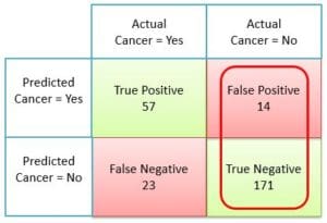
Specificity is the fraction of times the classifier predicts negatives cases correctly from the total number of actual negative cases. This metrics is the opposite of Recall/Sensitivity that we understood above.
Specificity = \(\frac { TN }{ TN+FP } \)
Here TN+FP is the total number of actual negative cases. If you are confused, just take a minute to observe the confusion matrix, you will realize this.
In our example, TN = 171 non-cancer cases were predicted correctly by the classifier and FP = 14 non-cancer cases were incorrectly identified as cancer. And the total non-cancer cases were TN+FP = 171+14 = 185.
Specificity = \(\frac { 171 }{ 171+14 } \) = \(\frac { 171 }{ 185 } \) = 0.92
So this means our model has 92% capability to identify negative cases from total number of actual negative cases.
Precision
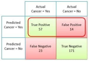
Precision calculates the fraction of times the model predicts positive cases correctly from the total number of positive cases it predicted.
Precision = \(\frac { TP }{ TP+FP } \)
Okay, so TP+FP is the total number of cases predicted by the classifier as positive. And TP is the total number of cases that are actually positive.
In our example, the classifier predicted TP+FP = 71 cases of cancer. Out of these 71 cases, only TP = 57 cases were correct.
Precision = \(\frac {57}{ 57+14 } \) = \(\frac {57}{ 71 } \) = 0.80
So this means our classifier has a precision or correctness of 80% when it predicts cases as cancer.
Recall Vs Precision
I will take a moment here to make you realize an interesting thing when it comes to Precision and Recall.
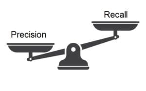
Ideally both Recall and Precision should be very high and as close to 100% as possible. But a machine learning classifier can start compromising with one or the other in achieving this high percentage for one of them (especially when data is imbalanced). Let me explain to you this.
- To achieve a high recall, our classifier can aggressively start identifying every other case as cancer so as to cover as many actual cancer cases as possible. With this tendency, it may predict almost all actual cancer cases (thus achieving high recall) but the prediction is also having way too many false positives also (thus achieving low precision).
- On the other hand, to achieve high precision, the classifier may classify only those cases as cancer for which it calculates very high probability. It does not classify those cases as cancer whose probability is not very high. With this conservative approach, almost all cases identified as cancer are actually correct (thus achieving high precision). But we might not be correctly predicting many other actual cancer cases (thus achieving low recall).
Ideally, a good classification model should be able to strike a balance between Precision and Recall without compromising one for the other.
F1 Score
As we saw above, you should keep a watch on both Recall and Precision when creating classification models. You might be creating multiple models and then comparing their precision and recall to choose the best among them. Will it not be great if we have just one metric to keep the evaluation and comparison process simple. Luckily we have an F1 score !!
F1 Score = \(\frac { 2*Precision*Recall }{ Precision+Recall } \)
As you can see, the F1 score is actually the harmonic mean of Precision and Recall. Using F1 scores you can now evaluate and compare the performance of the models easily now.
Bonus – Confusion Matrix for Multiple Classes
Yes, the confusion matrix exists for multiple classes also. It might look bigger depending on the number of classes but believe me it is very simple to understand. Let us understand this with an example of 3 class confusion matrix.
Let us assume we have a machine learning model that goes through several images of Dog, Cat, and Rabbit and classify them accordingly. This is how the confusion matrix looks like.
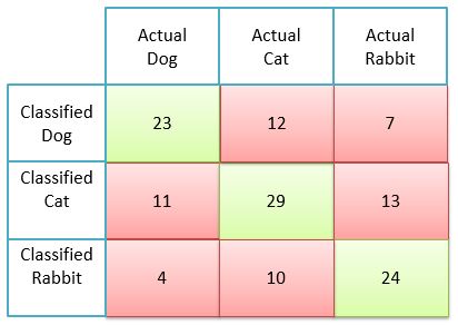
Here, the diagonal green squares are True Positive. For e.g. model classified 23 images as dogs and they were actually dogs.
The red squares are the miss classifications of our model. For e.g. out of all the images the model classified as Cat, 11 were actually dogs and 13 were actually Rabbit. Only 29 images were correctly classified as Cat.
I will suggest exploring this example with some focus and you will understand multi-class confusion matrix.
In The End …
I hope this article took your confusion out of the confusion matrix and helped you build an understanding of various metrics available to measure the performance of machine learning models.
Do share your feedback about this post in the comments section below. If you found this post informative, then please do share this and subscribe to us by clicking on the bell icon for quick notifications of new upcoming posts. And yes, don’t forget to join our new community MLK Hub and Make AI Simple together.


