Introduction

This is the first of the two-part series of the mini-project of retrieving relevant research papers from aRxiv dataset, based on the user’s query by using the topic modeling and cosine similarity.

 In this Part -1, we will focus on exploratory data analysis, visualization, and text preprocessing and get ready for Part -2.

The dataset for this example is available over Kaggle. You can download it from here. This dataset is a huge dataset in JSON format with information of over 24000 research papers. The research papers included in this dataset are starting from the year 1992 to the year 2018.

Custom Functions Overview

To have a quick overview, we have created below user-defined functions in our code that will work as pillars for the entire project.

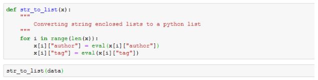
• str_to_list() – This function helps in converting string information into python lists.
• preprocess_text() – This function is used for preprocessing of text data.
• compute() – This function assists in calling the main functions, along with this by using the compute() function, we are storing the results obtained through our algorithms by using pickle.

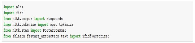
Loading Libraries

We will now start this tutorial by loading the required libraries. Here “pickle” library is used for storing the python objects in a file for the usage of results in related files. The library will store the results in a file with a “.pickle” extension.

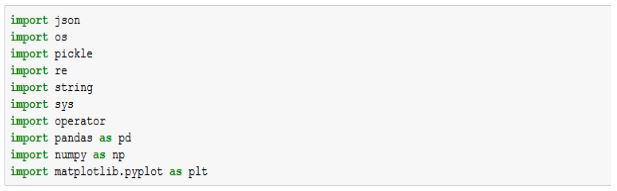
The other important libraries involve NLTK and fire, the main usage of “fire” is used to launch a python object in the command-line interface.

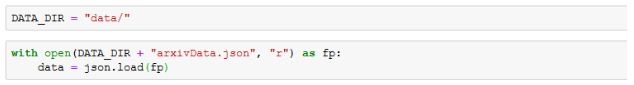
Loading Data

It’s time to load our research papers dataset by using the “open” function of python. Here the directory where the dataset is stored is provided in a variable. The dataset is stored in a folder titled “data”. The first python file is titled “preprocess”.

Here if we see the snapshot of the dataset obtained from the website, each value in the JSON file has 9 attributes defining each research paper.

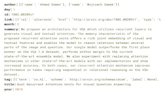
Using the below code, we are fetching the information of the author and tags of each research paper. The “str_to_list” function is passed the dataset stored in the “data” variable. In the function we have used the “eval” function, it helps in converting any string into a python list.

Exploratory Data Analysis and Data Visualization

Count of Research Paper Published Per Year

The first visualization is to look for the count of research papers published each year. For this, we are using a “for” loop where the count for each individual year is added, this will help in getting to know the number of publications each year.

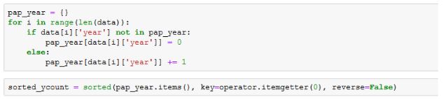
The “pap_year” list created with the for loop is then sorted for obtaining efficient results.

The visualization of “papers published in each year” is depicted using a bar graph, also known as count plot.

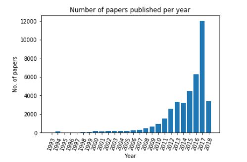
• Clearly, the highest number of research papers are published in the year 2017.
• This visualization also supports the fact that in the last decade, the popularity of Artificial Intelligence and its related fields has increased in a huge amount. 

This is one of the reasons why the count of research papers published has increased with each passing year. The year 2018 has lesser count because this dataset was compiled before the finishing of 2018. Otherwise, the same trend would have been visible.

Most Frequent Tags in Research Papers

The next visualization will tell us about the most frequent tags encountered in the dataset.

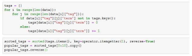
Here again, tags count is calculated using the “for loop”. Then the list containing the information is sorted and we fetch the ten most frequent or popular tags.

We have prepared a list of tags observed from the dataset and this list will then be used for visualization.

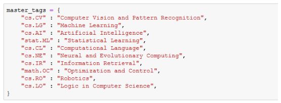
Finally, the visualization of the popular 10 tags is completed using a bar plot, built using the “barh” function (especially used for horizontal bar plot).

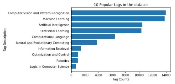
• The bar plot shows that “Computer Vision and Pattern Recognition” and “Machine Learning” are the two most occurring tags in the dataset.

Text Data Preprocessing

Now to perform the next visualization and also for getting further results, we will be executing text preprocessing of the data by using NLTK library and NLP methods.

First of all, the summary of each research paper is extracted in a list known as “summaries”. These are then joined together.

For the purpose of text data preprocessing, a function called “preprocess_text” is built which will be used for executing some of the basic operations which are necessary for text data cleaning and preprocessing.

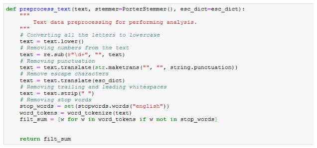
As we can see, the text is converted to lowercase for uniformity of operations and results. Using the regular expression, the numbers are removed. 

With the help of the “translate” function, all the unwanted punctuation and escape characters are removed. Once the strip function drops the whitespaces, the stopwords such as “a, an,the” are removed and words are tokenized.

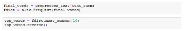
After building this function, the summaries which were joined above to create a list are passed as a parameter to “preprocess_text” function.

Frequently Occurring Words

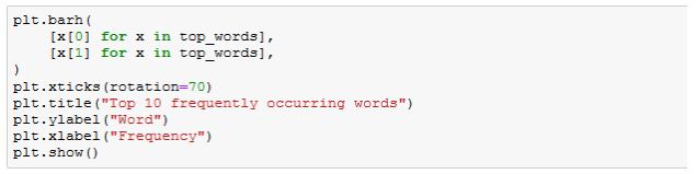
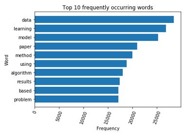
Then frequency is calculated for the top words obtained in the summaries. Again the top 10 commonly featuring words are visualized using the below code for horizontal bar plots.

So the below visualization shows that “data” and “learning” are stressed more by the researchers while writing the abstract.

Building TF-IDF Vectors

The next task in this tutorial is to generate the TF-IDF vector for summaries of each research paper. TF-IDF or Term Frequency – Inverse Document Frequency is a method that helps to know which words are of greater significance and which are less worthy based on the word’s frequency. 

In such documents, where there is a large chunk of text we cannot trust the method where words with high frequency decide the topic of the paper. So using the TF-IDF method, we give more weightage to the words which are less in count in the text and words with more count are considered useless.

Therefore, through the TF-IDF method, we’ll be representing each summary with the help of the TF-IDF vector, this vector will be saved using pickle and will then be used further.

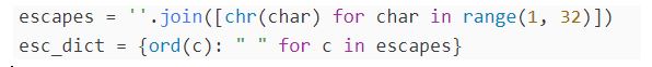
Here using the below code, a dictionary is created which will consist of all the characters, this dictionary will be used in the upcoming function.

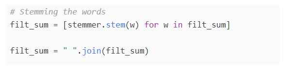
Stemming is a process used in NLP for extracting the root word and removing the suffixes attached to different words. This function should be included in the “preprocess_text” function, once the output for the most frequent word visualization is obtained. 

NOTE: Remember to include the below code after visualizing the most frequent word visualization, otherwise you may not get desired results.

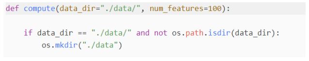
So to compute the TF-IDF vector mode, the “compute” function is created. The two parameters passed to this function will be the location of our dataset and the number of features. The “num_features” parameter is used to specify the number of words used for this function in a single execution.

The data location is provided through the “os” library. 

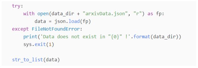
In the try…except block, we are loading the arxiv research papers dataset. The “str_to_list” is used for converting the string data into python lists.

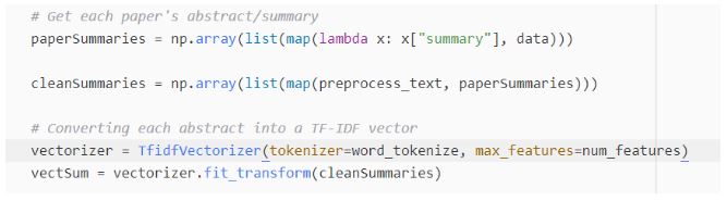
Now the summaries of all the research papers are combined into a list using the map function. This list is then cleaned and preprocessed using the “preprocess_text” function. After this, using “TfidfVectorizer”, the TF-IDF model is built and each research paper’s abstract is having its TF-IDF vector.

Text Preprocessing Research Papers Abstract

Lastly, using the pickle library we will be saving the results into two different pickle files. The first pickle file contains tf-idf vectors built using the “vectSum” variable and the other pickle file is built using “vectorizer”.

Saving the results

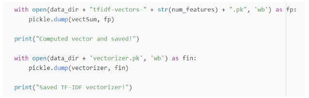
As an output, you would see “Computed vector and saved!” and then “Saved TF-IDF vectorizer”.

NOTE: These two pickle files will be stored in the same location where the dataset was stored.

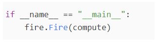
At last, to run the code, we will be using the “fire” library. Using this library, we can launch python objects such as lists, functions, etc. in command-line interface. 

Conclusion

Reaching the end of this tutorial, we have started a project based on clustering. In this article, we looked at the real-world implementation of clustering, with a major focus on clustering aRxiv research papers dataset obtained from Kaggle. After having covered various kinds of visualization for exploring and understanding the dataset. 

The tutorial also covers how each research paper’s abstract is converted into a TF-IDF vector for further processing. In the next article, we will see how we can do topic modeling and cluster the documents for information retrieval.