3 Examples of Monte Carlo Simulation in Python

Introduction

In this post, we will understand what is Monte Carlo Simulation, what are its typical steps along with benefits and limitations. We will also take a look at its real-world application followed by a few examples of Monte Carlo simulation in Python along with visualization for better clarity.

What is Monte Carlo Simulation

Monte Carlo simulation is a computational technique to approximate the behavior or output of a complex system or problem by repeated random sampling. This method relies on the Probability Theory concept of the Law of Large Numbers which states that if an experiment is repeated a large number of times then its average results will converge towards the expected value.

Steps in a Monte Carlo Simulation

1. Define Problem – The first step is to define the problem you want to solve or model its behavior. This involves specifying input variables, parameters, and the desired outcomes.
2. Generate Random Samples – In this step, you have to generate a large number of random samples for input variables. This is an important step and the quality of randomly sampled data will determine the accuracy of Monte Carlo simulation.
3. Run the Simulations- In this step, you have to use the above random samples and run them through simulations by using specialized software or programming languages like Python, Matlab, or R. Make sure to record the output of each simulation run.
4. Analyze Results –  Finally, in this step, you analyze the results of the simulation to estimate probabilities, averages, variances, and other statistical parameters.

Advantages

Monte Carlo Simulation has the following advantages –

• It helps to model the behavior of complex systems with approximation.
• It has a wide range of industry & real-world applications.
• It helps you with insights for risk assessment and decision-making.
• It can also help you with optimization and resource allocation.

Limitations

• This technique requires a substantial number of simulations to achieve accuracy.
• The results are very much dependent on the quality of input data which are randomly sampled.
• It can become computationally intensive for complex models.

Real-World Applications of Monte Carlo Simulation

Finance

In finance, Monte Carlo simulation is widely used for risk management, portfolio optimization, and option pricing. It helps investors and financial institutions in decision-making by modeling various market scenarios and simulating the impact of future uncertainty on their investments.

Engineering

In engineering, Monte Carlo simulation is used for designing reliable systems by helping in the assessment of the reliability and safety of structures. This method is widely used in aerospace, civil engineering, and manufacturing industries.

Science

Scientists use Monte Carlo simulation to model complex things like particle interactions in particle physics, the behavior of molecules in chemistry, and the spread of diseases in epidemiology, etc.

Business Operations

Monte Carlo simulation can play a crucial role in optimizing supply chains, project management, and resource allocation. Businesses use it to make data-driven decisions and identify areas where improvements are needed.

1) Monte Carlo Simulation in Python for Calculating Pi

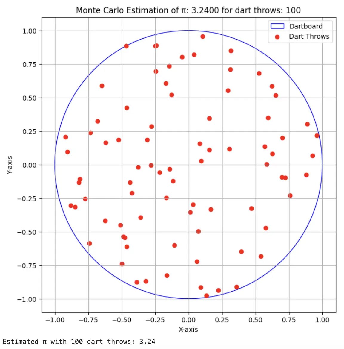
In this example, we are going to calculate the value of Pi with a Monte Carlo simulation in Python by playing a Dart game. For this, we simulate random throwing of dart within a unit square which encloses the unit circle representing our dartboard.

The ratio of the area of the unit circle to the area of the unit square is π/4. And the value of pi can be calculated as pi=4*total_points_inside_cicrle/total_points.

This entire experiment of Monte Carlo simulation is shown in below Python code. Here we first define the radius of the dartboard as 1 unit and the radius at (0,0).  Then we simulate dart throws by generating random coordinates between -1 and 1 and calculate if the dart throw is on the dart or not (i.e. within the circle or not). The number of dart throws simulation is controlled by variable num_dart.

After simulating all dart throws, the value of pi is calculated and the visualization is generated with the help of the matplotlib library.

In the first run, we run this code with simulation for only 100 dart attempts (num_darts = 100). From the output and visualization, we can see that the value of pi is close but not correct.

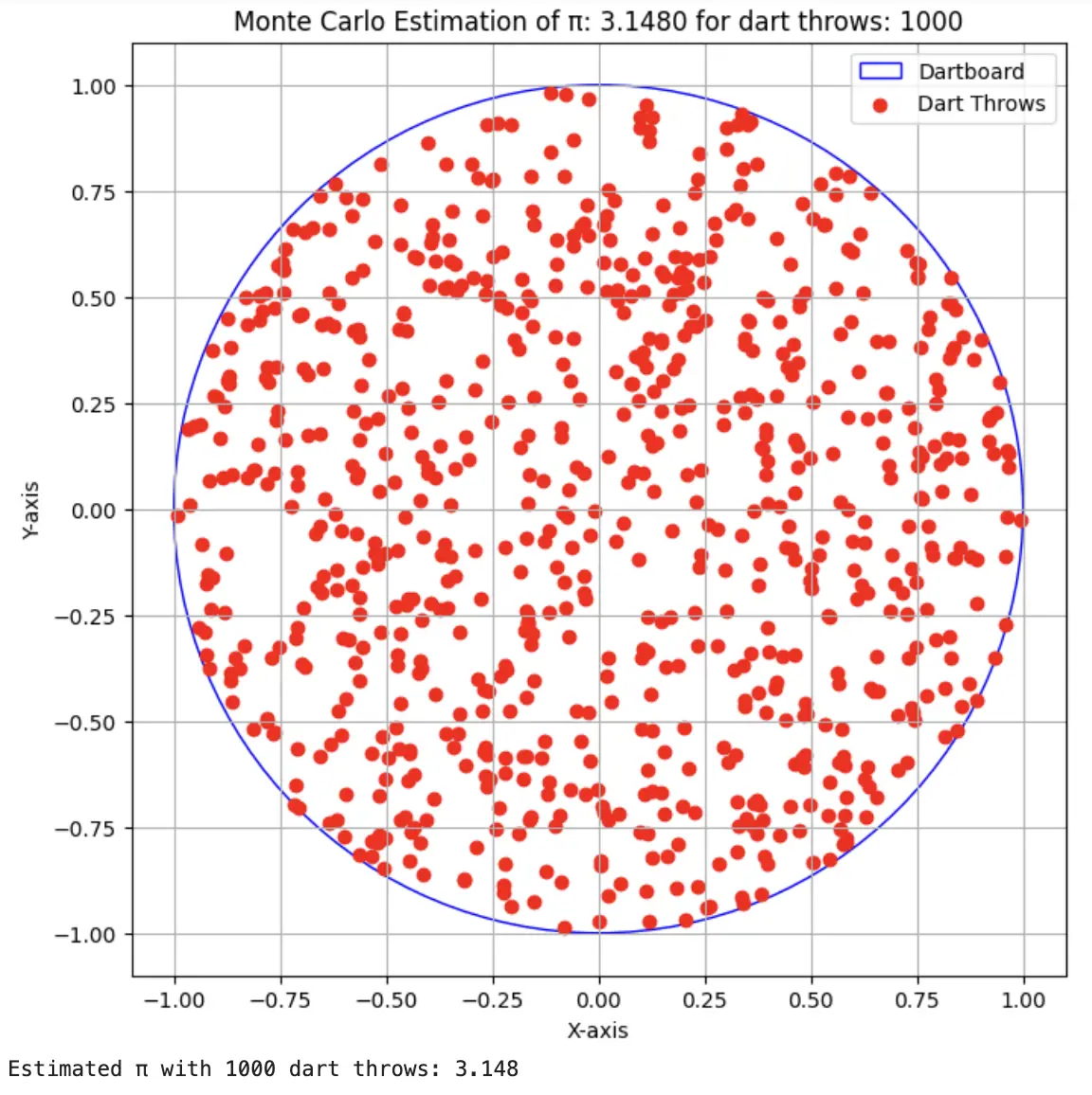
For the 2nd run, we use 1000 dart attempt simulations (num_darts = 1000). This time we can see from output and visualization we can see that the pi value has been approximated correctly. This shows that we have to run Monte Carlo simulations for a considerable number of time to converge to the expected output.

import random
import numpy as np
import matplotlib.pyplot as plt

def estimate_pi_with_dartboard_visualization(num_darts):
    inside_circle = 0
    x_inside, y_inside = [], []

    # Define the radius and center of the dartboard
    dartboard_radius = 1.0
    dartboard_center = (0, 0)

    for _ in range(num_darts):
        x = random.uniform(-dartboard_radius, dartboard_radius)
        y = random.uniform(-dartboard_radius, dartboard_radius)
        distance = x**2 + y**2

        if distance <= dartboard_radius**2:
            inside_circle += 1
            x_inside.append(x)
            y_inside.append(y)

    estimated_pi = 4 * inside_circle / num_darts

    # Visualization
    fig, ax = plt.subplots(figsize=(8, 8))
    circle = plt.Circle(dartboard_center, dartboard_radius, color='b', fill=False, label='Dartboard')
    ax.add_patch(circle)
    plt.scatter(x_inside, y_inside, color='r', marker='o', label='Dart Throws')
    plt.xlabel('X-axis')
    plt.ylabel('Y-axis')
    plt.title(f'Monte Carlo Estimation of π: {estimated_pi:.4f} for dart throws: {num_darts}')
    plt.legend(loc='upper right')
    plt.gca().set_aspect('equal', adjustable='box')
    plt.xlim(-dartboard_radius - 0.1, dartboard_radius + 0.1)
    plt.ylim(-dartboard_radius - 0.1, dartboard_radius + 0.1)
    plt.grid(True)
    plt.show()

    return estimated_pi

#First Run
num_darts = 100
estimated_pi = estimate_pi_with_dartboard_visualization(num_darts)
print(f"Estimated π with {num_darts} dart throws: {estimated_pi}")

#Second Run
num_darts = 1000
estimated_pi = estimate_pi_with_dartboard_visualization(num_darts)
print(f"Estimated π with {num_darts} dart throws: {estimated_pi}")

Output with num_darts = 100

Output with num_darts = 1000

2) Monte Carlo Simulation in Python for Dice Roll Probability

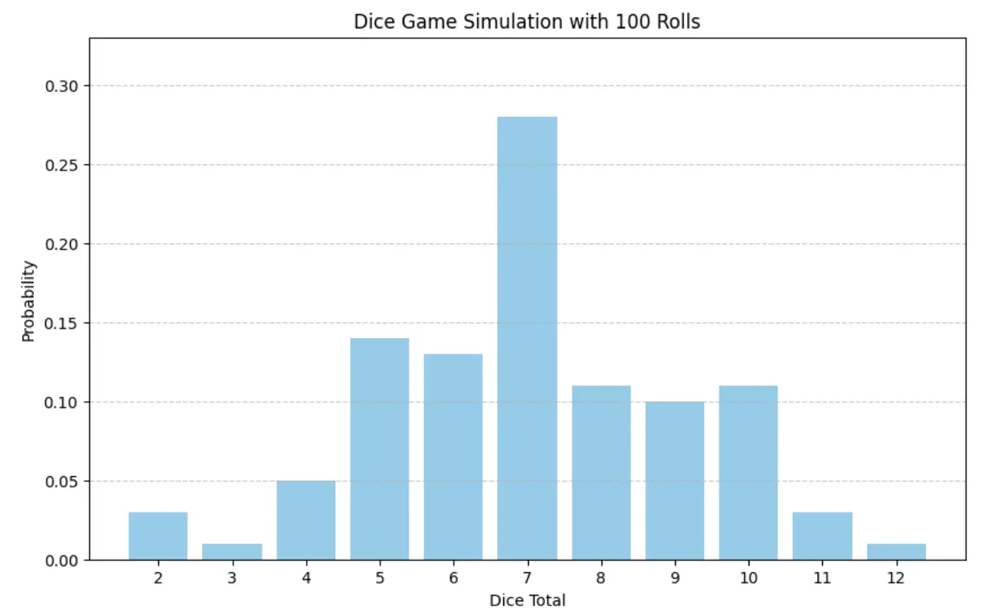
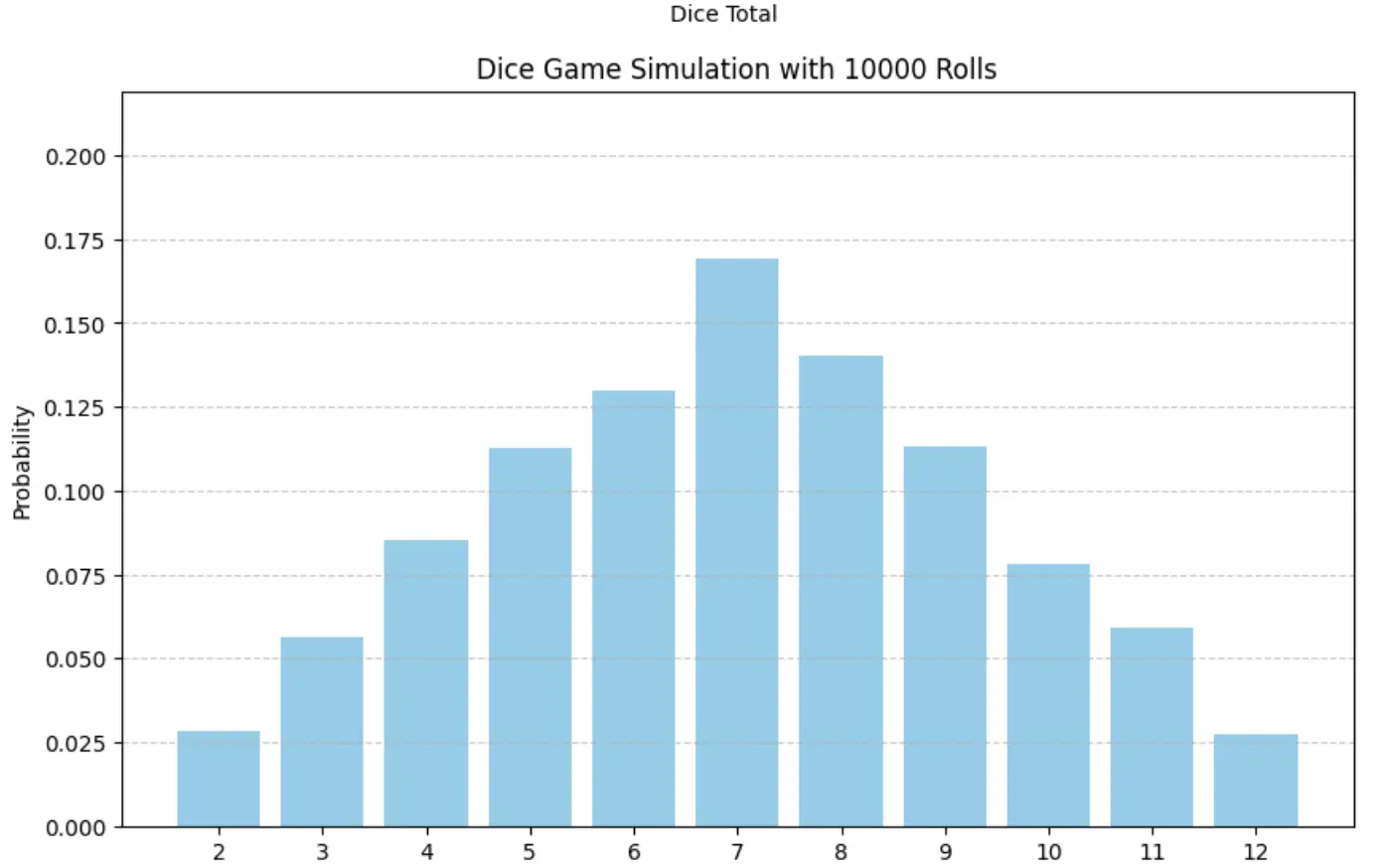
In this example, we are going to use Python Monte Carlo Simulation to predict the probability of the sum of two simultaneous dice rolls. The possible outcome value ranges from 2 to 12.  The purpose is to understand the probability distribution of the outcome by repeating dice rolls a considerable number of times.

In the below Monte Carlo Python simulation, we generate two random numbers between 1 and 6 corresponding to two dice rolls, and their sum is saved in each loop. After the simulation of the entire run, the probability of each possible value i.e. from 2 to 12 is calculated. Finally, the probability distribution is visualized with the help of a graph.

In the first run, we roll dice only 100 times i.e. we pass num_rolls = 100 and from the output graph we can see that probability distribution does not seem to have any known pattern.

In 2nd run, we roll dice 10000 times, i.e. we pass num_rolls = 10000 and this time from the output graph we can see that normal probability distribution appears, which is also known as Gaussian distribution.

import random
import matplotlib.pyplot as plt

def simulate_dice_game(num_rolls):
    outcomes = [0] * 11  # List to track the frequency of each possible outcome (2 to 12)

    for _ in range(num_rolls):
        dice1 = random.randint(1, 6)
        dice2 = random.randint(1, 6)
        total = dice1 + dice2
        outcomes[total - 2] += 1

    probabilities = [count / num_rolls for count in outcomes]

    # Visualization
    outcomes_labels = [str(i+2) for i in range(11)]
    plt.figure(figsize=(10, 6))
    plt.bar(outcomes_labels, probabilities, color='skyblue')
    plt.xlabel('Dice Total')
    plt.ylabel('Probability')
    plt.title(f'Dice Game Simulation with {num_rolls} Rolls')
    plt.ylim(0, max(probabilities) + 0.05)
    plt.grid(axis='y', linestyle='--', alpha=0.7)
    plt.show()

    return outcomes, probabilities

#First Run
num_rolls = 100
outcomes, probabilities = simulate_dice_game(num_rolls)

#Second Run
num_rolls = 10000
outcomes, probabilities = simulate_dice_game(num_rolls)

Output with num_rolls = 100

Output with num_rolls = 10000

3) Monte Carlo Simulation in Python for Integration Problem

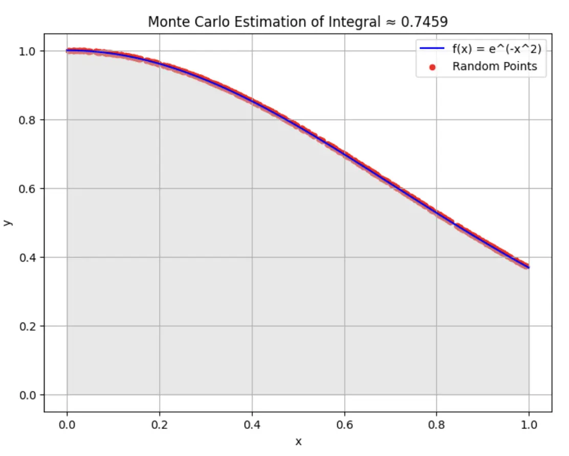
In this example, we are going to use Monte Carlo Simulation in Python to estimate the integral of function f(x) = e^(-x^2) over the interval [0,1].  This integral does not have a simple closed-form solution, making it a good choice for Monte Carlo integration.

In the below Python Monte Carlo Simulation code we first create a function f(x) that calculates the integral of f(x) = e^(-x^2) for a given value of x. Then random values are generated between the interval [0,1] and its actual and value and the estimated value is visualized on the graph.

For the first run for num_points=50, we can see that the points are somewhat aligned over the actual graph of (x) = e^(-x^2).

For the second run for num_points=100, it can be seen from the graphs that the approximation of integration of function f(x) = e^(-x^2)  is converging properly over the expected graph.

import random
import numpy as np
import matplotlib.pyplot as plt

def monte_carlo_integration(num_points):
    # Function to estimate the integral of: f(x) = e^(-x^2)
    def f(x):
        return 2.71828**(-x**2)

    # Interval for the integral: [0, 1]
    a, b = 0, 1

    # Initialize variable to store the integral estimate
    integral_estimate = 0

    # Lists to store random points for visualization
    x_points = []
    y_points = []

    # Perform the Monte Carlo simulation
    for _ in range(num_points):
        x = random.uniform(a, b)
        y = f(x)
        integral_estimate += y
        
        x_points.append(x)
        y_points.append(y)

    # Calculate the estimated integral value
    integral_estimate *= (b - a) / num_points

    # Generate x values for plotting the function
    x_values = np.linspace(a, b, 400)
    y_values = [f(x) for x in x_values]

    # Plot the function and the random points (larger size)
    plt.figure(figsize=(8, 6))
    plt.plot(x_values, y_values, label='f(x) = e^(-x^2)', color='blue')
    plt.scatter(x_points, y_points, color='red', s=20, label='Random Points')
    plt.fill_between(x_values, y_values, color='lightgray', alpha=0.5)
    plt.xlabel('x')
    plt.ylabel('y')
    plt.title(f'Monte Carlo Estimation of Integral ≈ {integral_estimate:.4f}')
    plt.legend()
    plt.grid(True)
    plt.show()

# First Run
num_points = 50
monte_carlo_integration(num_points)

# Second Run 
num_points = 500
monte_carlo_integration(num_points)

Output with num_points = 50

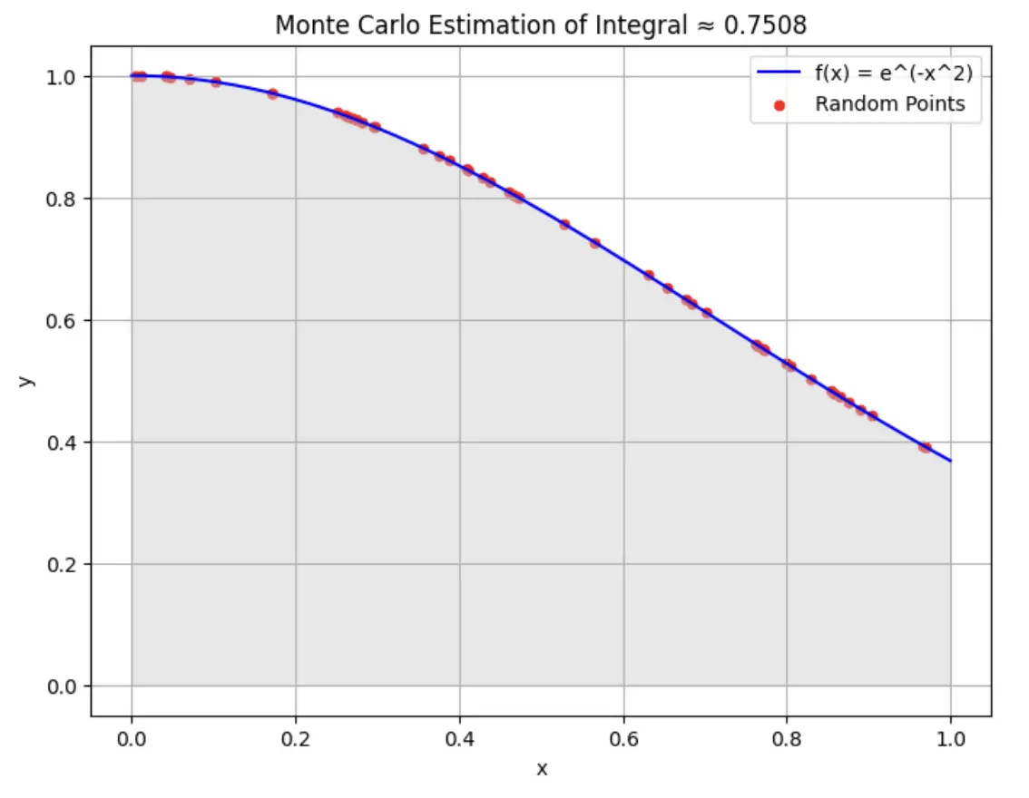
Output with num_points = 500