3 Common Techniques of Similarity and Distance Measure in Machine Learning

Introduction

In machine learning more often than not you would be dealing with techniques that requires to calculate similarity and distance measure between two data points. Distance between two data points can be interpreted in various ways depending on the context. If two data points are closer to each other it usually means two data are similar to each other.

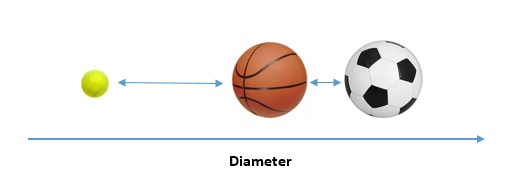
For e.g. if we are calculating diameter of balls, then distance between diameter of a basketball and diameter of a football will be less. This denotes that in terms of size both basketball and football are similar.

Whereas if we calculate diameter of tennis ball, then its distance with diameter of basketball and football will be larger. This denotes that tennis ball is not similar to either basketball or football in terms of size.

This example is visualized in one dimensional scale below –

Let us now look at common techniques of calculating distances between data points. The examples would be shown in 2 dimensional scale with two coordinates (x,y) but the technique can be extended to more dimensions.

• Also Read- How to deal with missing data in machine learning
• Also Read- Types of Data in Statistics – A basic understanding for Machine Learning

Manhattan Distance

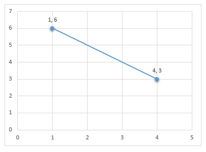
In this technique the Manhattan distance between two points are calculated as –

1. Take absolute difference between x coordinates of two points: |1-4| = 3
2. Take absolute difference between y coordinates of two points: |6-3| = 3
3. Take the sum of these differences : 3 + 3 = 6

Manhattan distance is also known as L1-Norm distance or absolute distance.

Euclidean Distance

In this technique, Euclidean distance between two points are calculated as –

1. Take the square of the difference between x coordinates of two points: \({ (1-4) }^{ 2 }\)
2. Take the square of the difference between y coordinates of two points: \({ (6-3) }^{ 2 }\)
3. Take the sum of the above two squares and then take it’s square root:\( \sqrt { { (1-4) }^{ 2 }+{ (6-3) }^{ 2 } } =\quad 4.24 \)

Euclidean distance is also known as L2-Norm distance

Cosine Similarity

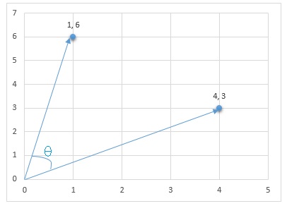
In this technique, the data points are considered as vectors that has some direction. The intuitive idea behind this technique is the two vectors will be similar to each other if the angle ‘theta’ between the two is small. On the other hand if the angle theta is more this means the two vectors are more distant apart and has less similarity or may be completely dissimilar.To measure this we calculate cosine of theta, hence the name Cosine Similarity.

When theta=0 then Cos 0 = 1 , therefor for two vectors to be similar the cosine theta should be closer to 1.

Let us see how to calculate cosine similarity for above example.

1. Multiply corresponding x and y coordinates of the two vectors and sum them: \(1*4\quad+\quad6*3\)
2. Take the square of each coordinates of first vector , sum them and then square root it: \(\sqrt { { 1 }^{ 2 }+{ 6 }^{ 2 } } \)
3. Take the square of each coordinates of second vector , sum them and then square root it: \(\sqrt { { 4 }^{ 2 }+{3}^{ 2 } } \)
4. Then the cosine similarity will be calculated as : \(\frac { 1*4\quad +\quad 6*3 }{ \sqrt { { 1 }^{ 2 }+{ 6 }^{ 2 } } *\sqrt { { 4 }^{ 2 }+{ 3 }^{ 2 } } } = 0.72\)

Points to Consider

Before we finish this article, let us take a look at following points

• In machine learning, Euclidean distance is used most widely and is like a default. So if it is not stated otherwise, a distance will usually mean Euclidean distance only.
• Manhattan distance also finds its use cases in some specific scenarios and contexts  – if you are into research field you would like to explore Manhattan distance instead of Euclidean distance.
• Cosine similarity is most useful when trying to find out similarity between two documents.
• All these are mathematical concepts and has applications at various other fields outside machine learning
• The examples shown here are for two dimension data for ease of visualization and understanding but these techniques can be extended to any number of dimensions
• There are other techniques also to find distance similarity between data, but these are very basic ones.

In The End …

Hope this was a good simple read with some fruitful insight, especially for beginners to understand similarity and distance measure in machine learning.

Do share your feed back about this post in the comments section below. If you found this post informative, then please do share this and subscribe to us by clicking on bell icon for quick notifications of new upcoming posts.