
Introduction
In this article, we will go through the tutorial on Keras LSTM Layer with the help of an example for beginners. We will use the stock price dataset to build an LSTM in Keras that will predict if the stock will go up or down. But before that let us first what is LSTM in the first place.
What is LSTM?
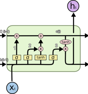
Long Short-Term Memory Network or LSTM, is a variation of a recurrent neural network (RNN) that is quite effective in predicting the long sequences of data like sentences and stock prices over a period of time.
It differs from a normal feedforward network because there is a feedback loop in its architecture. It also includes a special unit known as a memory cell to withhold the past information for a longer time for making an effective prediction.
In fact, LSTM with its memory cells is an improved version of traditional RNNs which cannot predict using such a long sequence of data and run into the problem of vanishing gradient.
Keras LSTM Layer Example with Stock Price Prediction
In our example of Keras LSTM, we will use stock price data to predict if the stock prices will go up or down by using the LSTM network.
Loading Initial Libraries
First, we’ll load the required libraries.
import numpy as np
import matplotlib.pyplot as plt
import pandas as pd
Loading the Dataset
We will now load the dataset, and we will use the head command to get an idea of its content.
dataset_train = pd.read_csv('NSE-TATAGLOBAL.csv')
dataset_train.head()
training_set = dataset_train.iloc[:, 1:2].values
Feature Scaling
To produce the best-optimized results with the models, we are required to scale the data. For this task, we are leveraging scikit-learn library’s minmax scaler for converting the input values between 0 to 1.
from sklearn.preprocessing import MinMaxScaler

sc = MinMaxScaler(feature_range = (0, 1))
training_set_scaled = sc.fit_transform(training_set)
Creating Data with Timesteps
When we are working with LSTM’s, we need to keep the data in a specific format. Once the data is created in the form of 60 timesteps, we can then convert it into a NumPy array. Finally, the data is converted to a 3D dimension array, 60 timeframes, and also one feature at each step.
X_train = []
y_train = []
for i in range(60, 2035):
    X_train.append(training_set_scaled[i-60:i, 0])
    y_train.append(training_set_scaled[i, 0])
X_train, y_train = np.array(X_train), np.array(y_train)

X_train = np.reshape(X_train, (X_train.shape[0], X_train.shape[1], 1))
Loading Keras LSTM and Other Modules
Now it’s time to build our LSTM, for this purpose we will load certain Keras modules – Sequential, Dense, LSTM, and Dropout.
from keras.models import Sequential
from keras.layers import Dense
from keras.layers import LSTM
from keras.layers import Dropout
Building the LSTM in Keras
First, we add the Keras LSTM layer, and following this, we add dropout layers for prevention against overfitting.
For the LSTM layer, we add 50 units that represent the dimensionality of outer space. The return_sequences parameter is set to true for returning the last output in output.
For adding dropout layers, we specify the percentage of layers that should be dropped. The next step is to add the dense layer. At last, we compile the model with the help of adam optimizer. The error is computed using mean_squared_error.
Finally, the model is fit using 100 epochs with a batch size of 32.
regressor = Sequential()

regressor.add(LSTM(units = 50, return_sequences = True, input_shape = (X_train.shape[1], 1)))
regressor.add(Dropout(0.2))

regressor.add(LSTM(units = 50, return_sequences = True))
regressor.add(Dropout(0.25))

regressor.add(LSTM(units = 50, return_sequences = True))
regressor.add(Dropout(0.25))

regressor.add(LSTM(units = 50))
regressor.add(Dropout(0.25))

regressor.add(Dense(units = 1))

regressor.compile(optimizer = 'adam', loss = 'mean_squared_error')

regressor.fit(X_train, y_train, epochs = 100, batch_size = 32)
Predicting Future Stock using the Test Set
Now we’ll import the test set for performing the predictions.
dataset_test = pd.read_csv('tatatest.csv')
real_stock_price = dataset_test.iloc[:, 1:2].values
For predicting the stock prices, firstly the training set and test set should be merged. The timestep is set to 60, we also apply MinMaxScaler on the new dataset and lastly, the dataset is reshaped.
We are required to use inverse_transform for obtaining the stock prices.
dataset_total = pd.concat((dataset_train['Open'], dataset_test['Open']), axis = 0)
inputs = dataset_total[len(dataset_total) - len(dataset_test) - 60:].values
inputs = inputs.reshape(-1,1)
inputs = sc.transform(inputs)
X_test = []
for i in range(60, 76):
    X_test.append(inputs[i-60:i, 0])
X_test = np.array(X_test)
X_test = np.reshape(X_test, (X_test.shape[0], X_test.shape[1], 1))
predicted_stock_price = regressor.predict(X_test)
predicted_stock_price = sc.inverse_transform(predicted_stock_price)
Plotting the Results
Let us plot the results of stock prices with the help of matplotlib library.
plt.plot(real_stock_price, color = 'black', label = 'TATA Stock Price')
plt.plot(predicted_stock_price, color = 'green', label = 'Predicted TATA Stock Price')
plt.title('TATA Stock Price Prediction')
plt.xlabel('Time')
plt.ylabel('TATA Stock Price')
plt.legend()
plt.show()
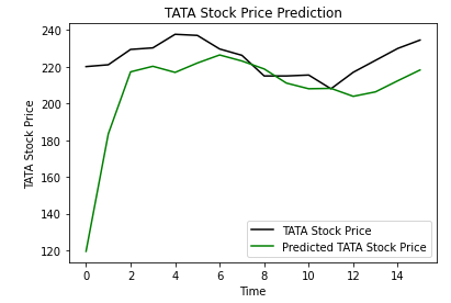
The above plot shows that Tata Stock Price will go up and our model prediction also shows that the price of Tata Stock will go up. This shows how well we have trained our model for time series and sequential problems.
- Also Read – Different Types of Keras Layers Explained for Beginners
- Also Read – Keras Dropout Layer Explained for Beginners
- Also Read – Keras Dense Layer Explained for Beginners
- Also Read – Keras Convolution Layer – A Beginner’s Guide
- Also Read – Beginners’s Guide to Keras Models API
- Also Read – Types of Keras Loss Functions Explained for Beginners
Conclusion
Now we will end this tutorial where we looked at the Keras LSTM Layer implementation. We learned how we can implement an LSTM network for predicting the prices of stock with the help of Keras library. The LSTM powered model was trained to know whether prices of stock will go up or down in the future.
Reference Keras Documentation

